The problem with tunnels and stairs

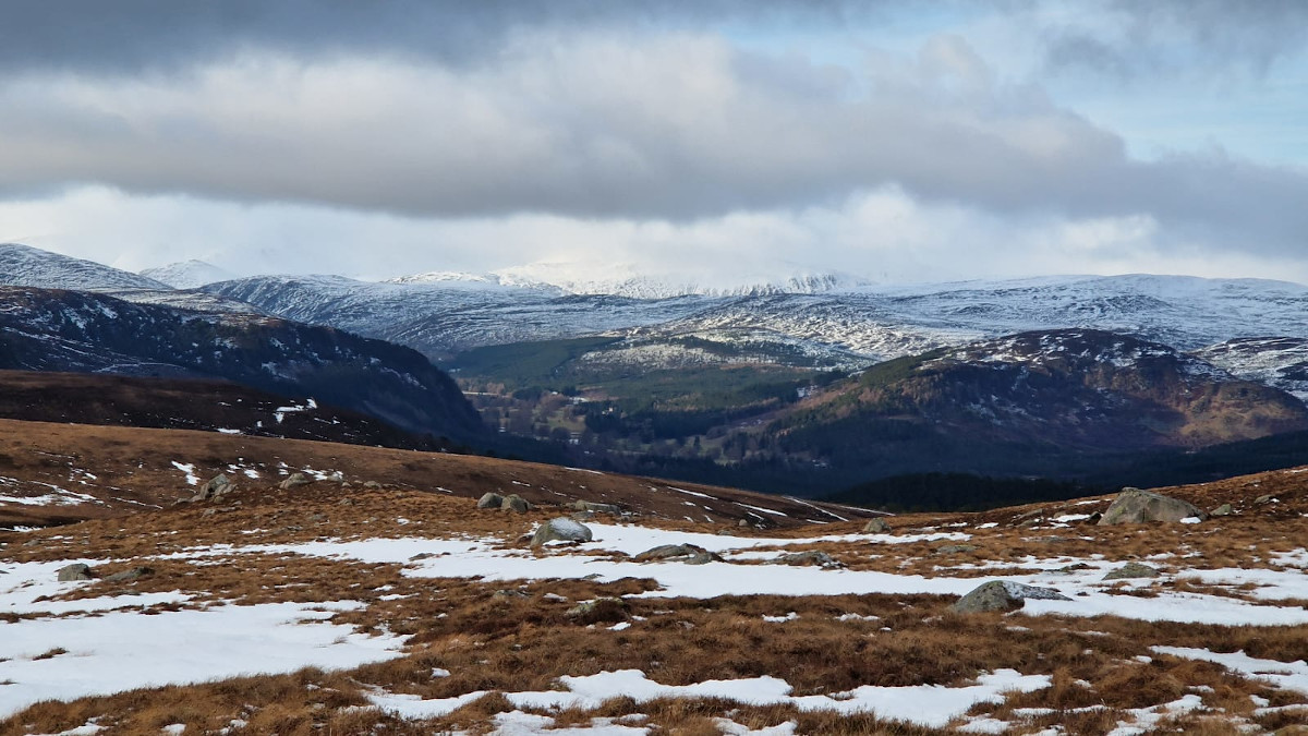
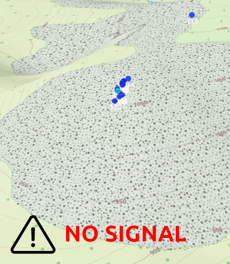
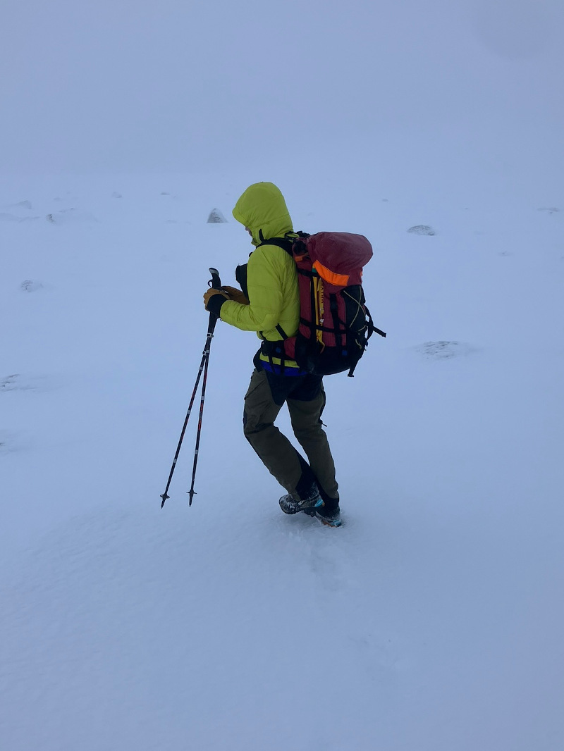
Whenever there’s been a major incident involving emergency services in complex urban environments the inquiry report has consistently highlighted radio communications failure despite significant developments in radio communications and 3D technology since the infamous 1988 Kings Cross Fire on the London Underground. The following tragic incidents all featured tunnels, stairs and communications failure:

• The 1988 Kings Cross Fire report highlighted radio communications only worked when they were in line of sight.
• The 2007 London underground bombings report highlighted that radio communications from trains to network control were inadequate or non-existent.
• The 2017 Grenfell tower fire inquiry highlighted inadequate radio communications between the incident control on the ground floor and fire fighters higher up the tower.

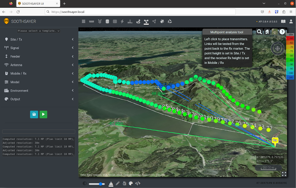
Limitations of (2D) radio planning tools

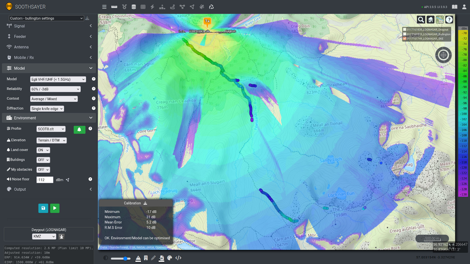
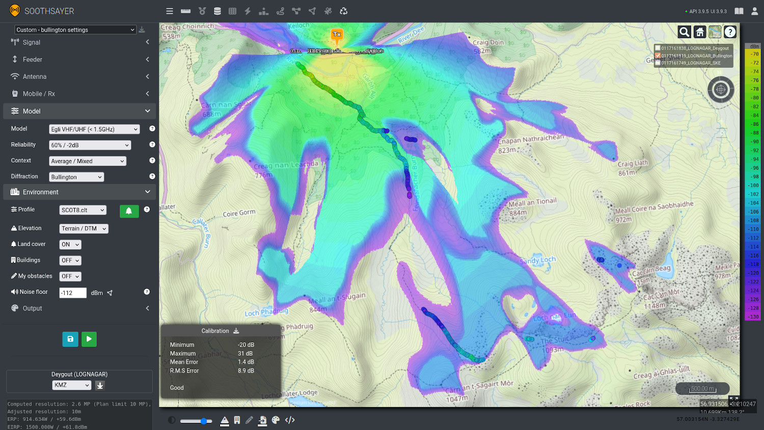
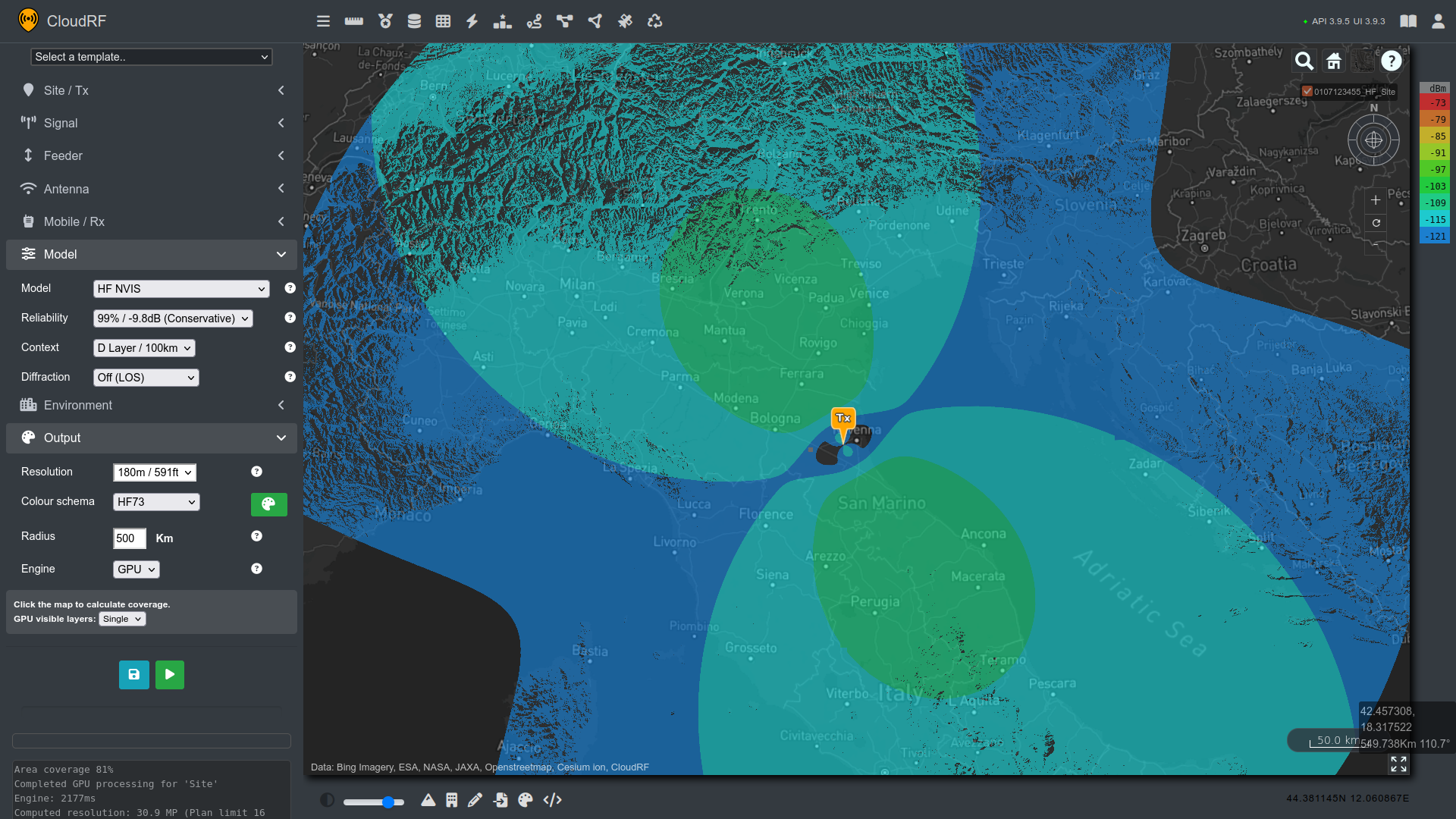
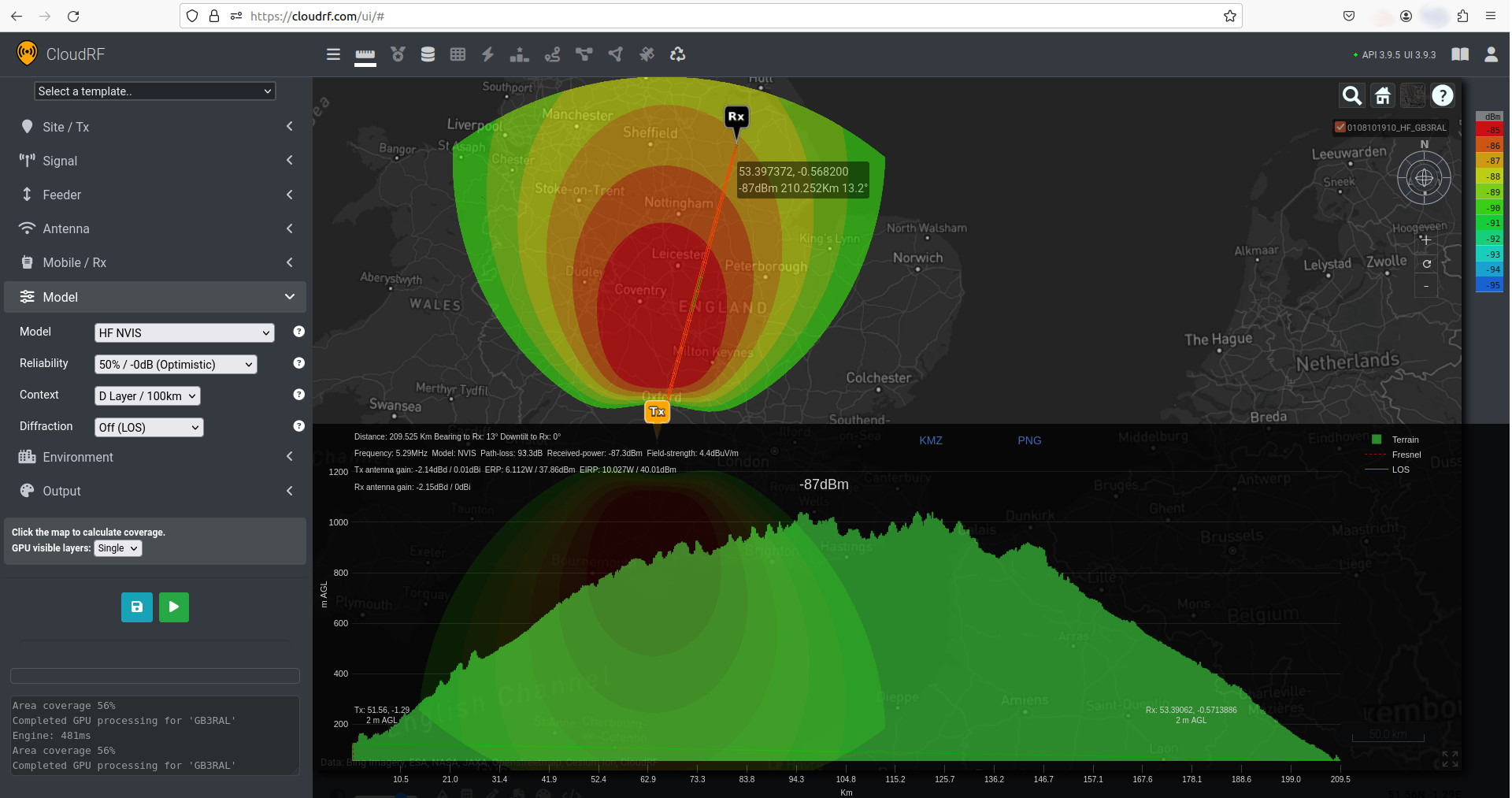
Radio planning tools are not used in emergencies. They’re complicated, slow and require a lot of knowledge to produce an accurate output. Even if a skilled operator were able to model a site before the event, currently they would be expected to model each floor of a multi-story building in isolation due to the “floorplan” design of current software.

The problem is indoor planning tools are built for corporate clients to achieve seamless Wi-Fi in every corner of the office, not to help a fire chief deploy a mesh radio network down stairs and then along a tunnel. The top end tools can do limited multipath, slowly, but not as an API which can be consumed by a third party viewer…

Most radio planning tools on the market, ourselves included, have the following limitations when it comes to complex urban modelling which we will explore in detail:

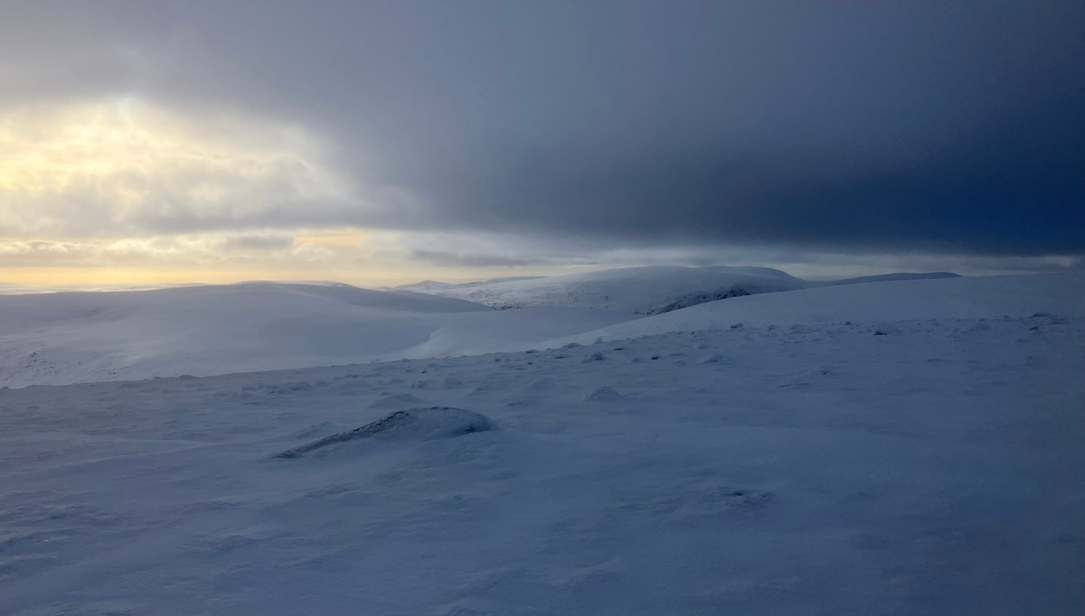
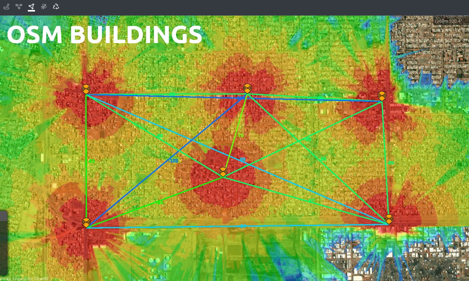
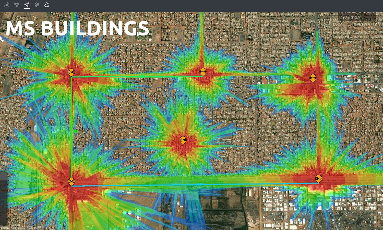
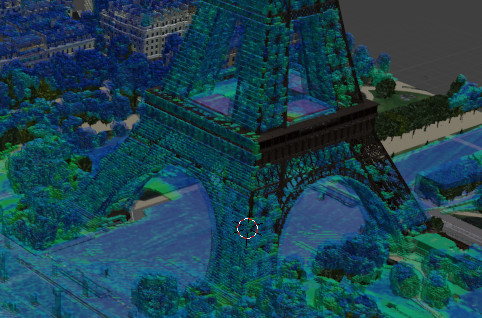
Using LiDAR as a 2.5D surface model

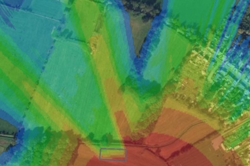
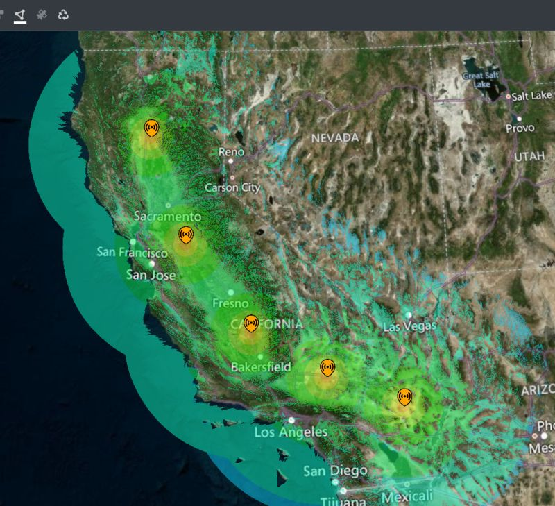
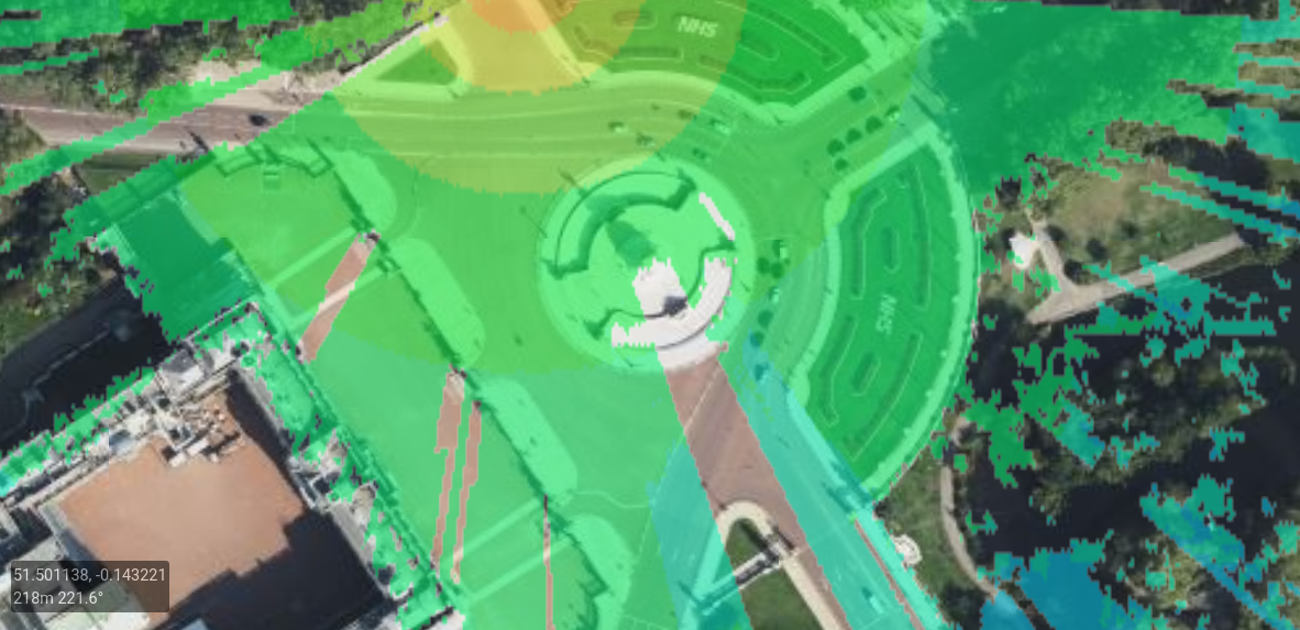
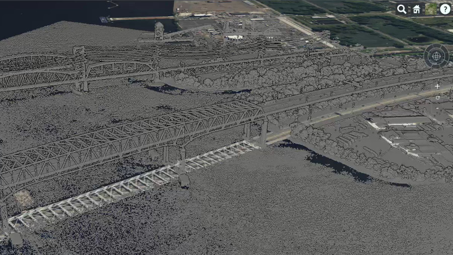
The abundance of free LiDAR data has made this high resolution data the standard for accurate outdoor RF planning and for several Fixed Wireless Access (FWA) tools, including free LiDAR based path tools, it is their core feature. We started using LiDAR in 2015 and know its limitations well; for example when point cloud LiDAR has been rasterised into GeoTIFF then it’s no longer 3D, it’s a 2.5D surface model which is useful for building heights and unsuitable for bridges, arches and tunnels.

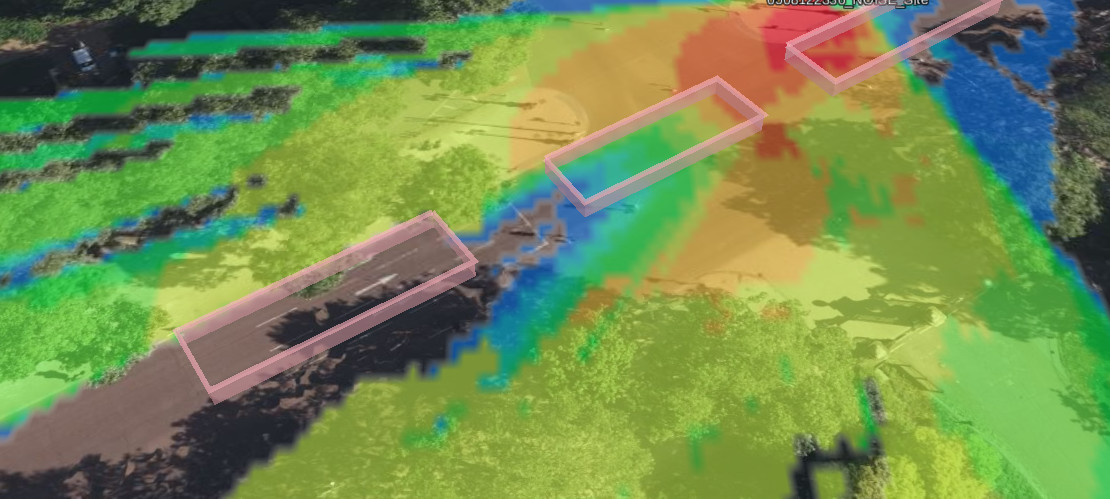
A bridge or arch in a rasterised LiDAR model extends to the ground like a wall. In the screenshot below, a large ferris wheel is blocking line of sight through it as well as the elevated rail bridge across the river which is casting a shadow much larger than it would in reality.

Using a floor plan to model a building

For indoor Wi-Fi planning tools, the start point is typically a floor plan. This does not scale well with multi-story buildings or support vertical planning as it produces a 2D image of a 2D plan.

Many tools present 2D images in a 3D viewer, as we do, but the output remains 2.5D, as with rasterised LiDAR. The significant Wi-Fi attenuation presented by solid floors makes this simplified 2D floor-by-floor planning viable for corporate clients in offices but not in challenging environments or where a floor plan does not exist.

Direct ray only

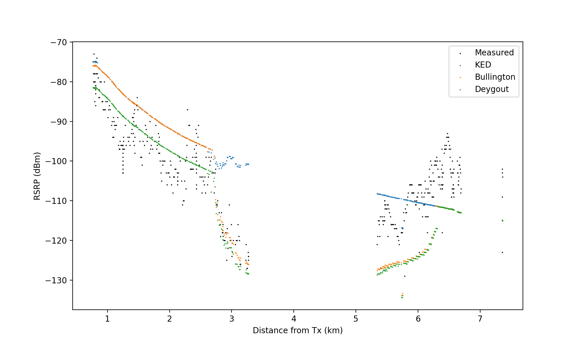
Modelling multipath, or fast fading, is much more complex than the direct ray. For this reason, most tools only do the more powerful direct ray and even then some cannot do diffraction or obstacle attenuation as we do already. For the previously mentioned Wi-Fi planning tools, the current standard is to model obstacle attenuation only. By doing this a tool is able to simulate most of the coverage quickly for a given floor but for complete accuracy it must be augmented by a walk survey, which isn’t so quick. For some customers, a walk survey is just not possible.

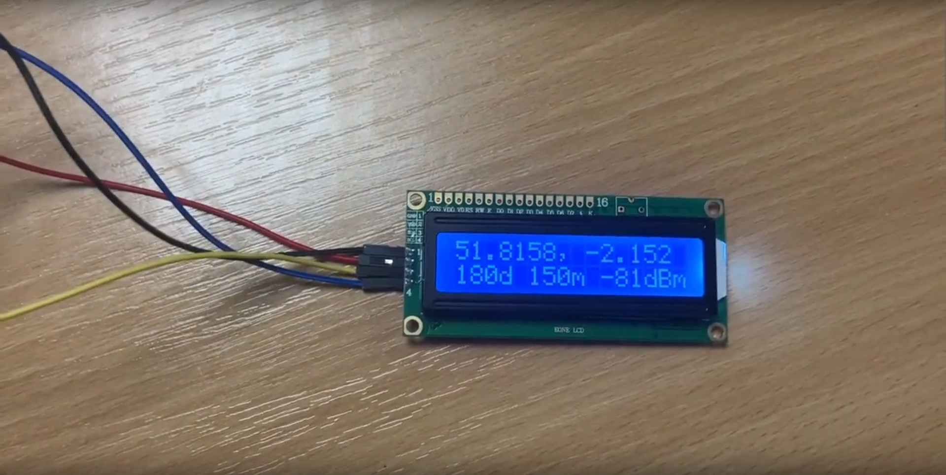
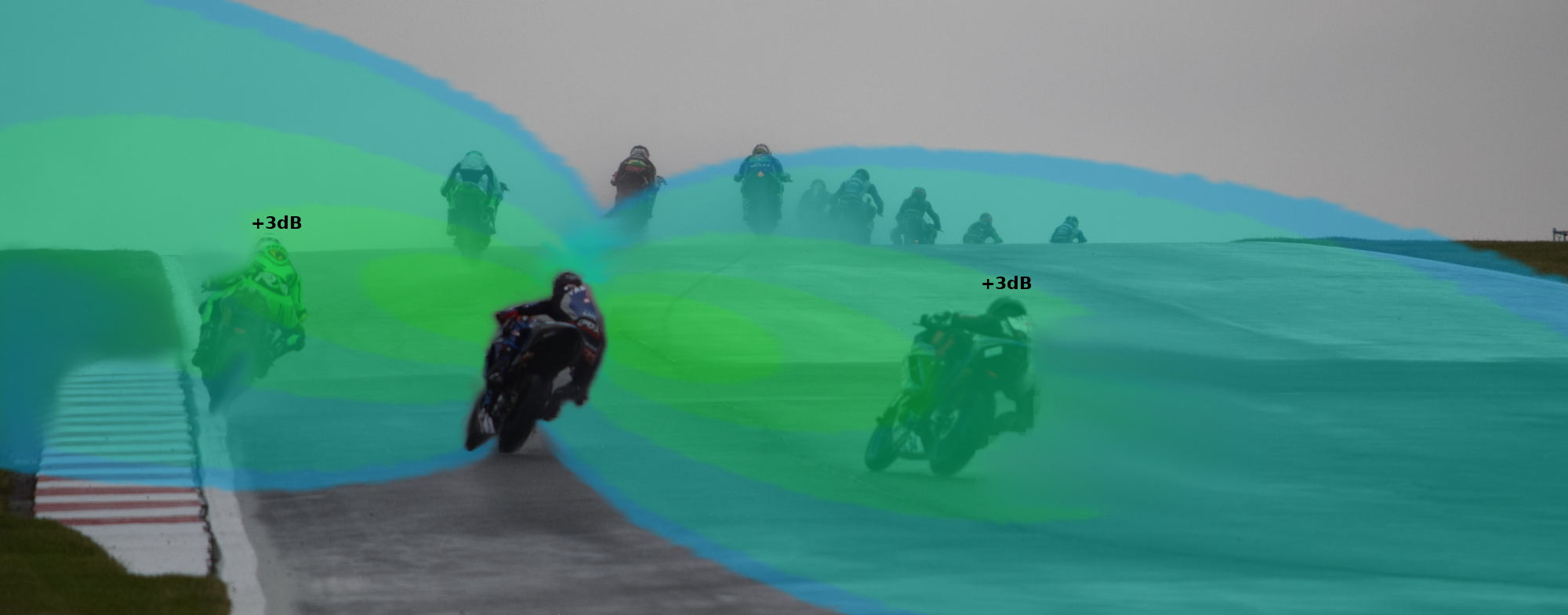
Multipath effects will increase coverage beyond a direct ray simulation and cause phase issues like signal dead-spots and doppler spread where reflections increase bandwidth and overall noise. This effect can be observed indirectly via customer reviews for urban WISPs where people state their once good link quality reduced as more neighbours subscribed.

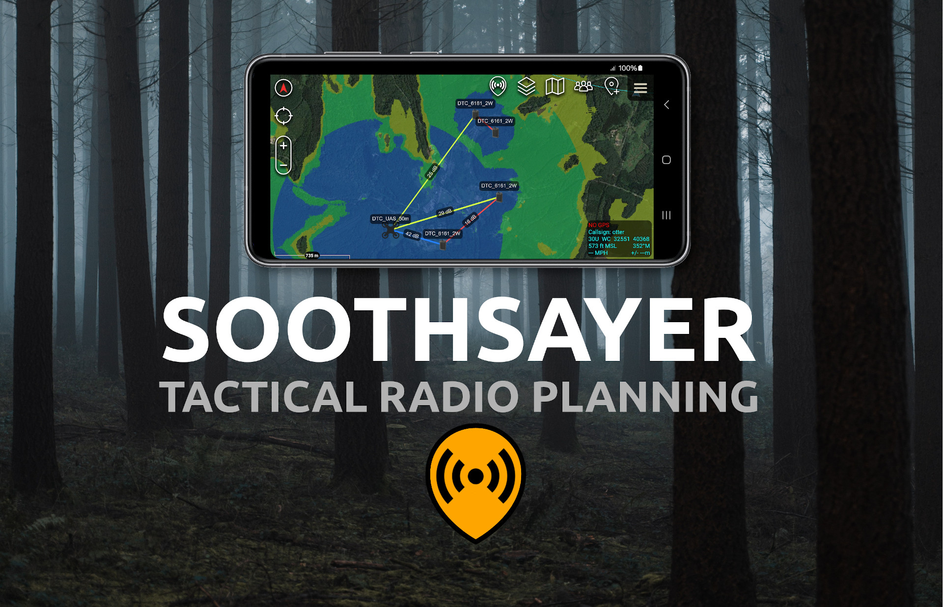
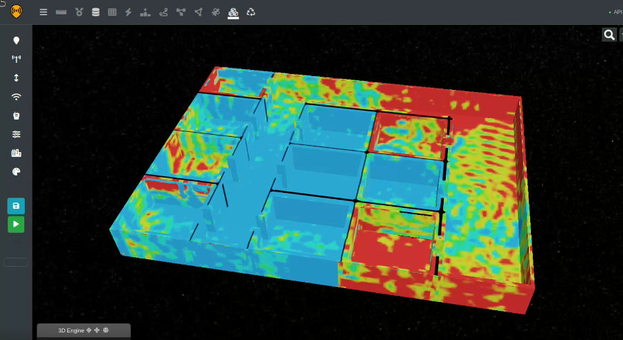
A 3D multipath API for 2024

We’ve been working on this full 3D capability since the 2022 Grenfell inquiry with valuable input from firefighters, mining experts and MANET radio OEMs. The first version of the engine is done and we’re onto API integration now.

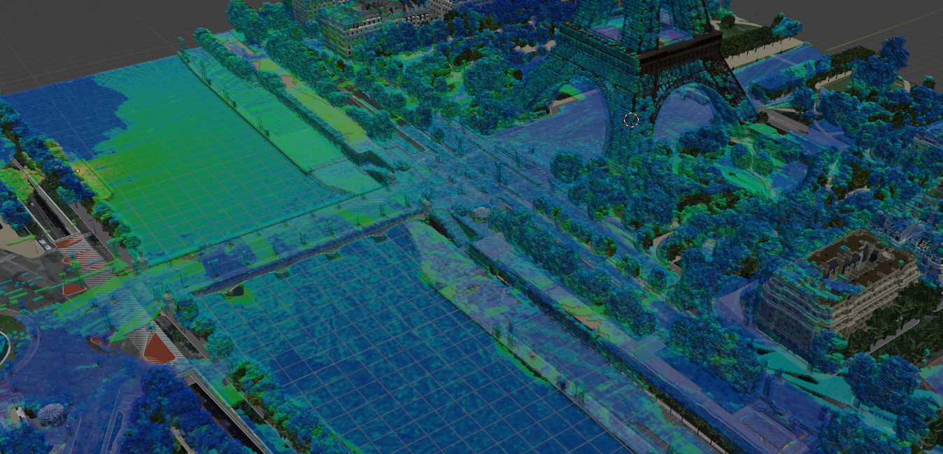
Our GPU based design takes a 3D model, simulates propagation in all directions irrespective of floors including configurable reflections, surface refractivity, material attenuation and crucially it outputs to the open 3D standard glTF. It scales from small rooms to suburbs and everything in between so will be used for tunnels, multi-story buildings and outdoor multipath.

It will be integrated into our API first so other standards compliant viewers can visualise it and will then be integrated into our own 3D user interface. We can’t say what interfaces people will be using in the future but are confident that by aiming for open standards APIs we will ensure compatibility with phones, glasses and holograms.

Done

Read LiDAR into a 3D volume

Prepare a volume from a LAS/LAZ LiDAR scan.

Done

Direct ray with attenuation

Model direct ray with configurable attenuation in dB/m for obstacles

Done

Reflections

Model reflections accurately based on the wavelength and angle of incidence

Done

Phase tracking

Track the phase to show constructive and destructive interference (fast fading) eg. dead spots, cured by a little movement 😉

Done

BIM / glTF support

Read and write BIM models as the open standard glTF “3d tiles” format.

Under development

API integration

Integrate engine into the CloudRF API so a BIM/LAS model can be uploaded and used via our standard JSON requests.

Under development

3D tiles web interface integration

Add 3D tiles output to 3D web interface. Some interfaces already supported 🙂

To do

Multisite support

Model many sites at once

To do

Antenna pattern integration

Add 3D antenna pattern loss

Commercial plan

The 3D engine API will be a new feature within CloudRF Gold plans and our SOOTHSAYER server at no additional cost. It requires a GPU. We’re aiming to get a beta up on CloudRF in May/June and to ship this with the next major SOOTHSAYER release, currently scheduled for September.

Users will be allowed to upload models within their storage limits and execution time / accuracy will be scaled to fit within a reasonable time. Limits will be relaxed on SOOTHSAYER.

We are partnering with open standards based companies to integrate this into different viewers. One exciting partner we are working with now is Avalon Holographics. Their revolutionary display is able to display our rich engine output in a hologram format so it can be explored in three dimensions for maximum spatial awareness without additional hardware for viewers.

If you would like to get our open standard glTF models into your viewer, get in touch. If you can bring challenging BIM models or LiDAR scans of real tunnels and large buildings we would really like to talk to you.

Demo video

Recently, we added advanced diffraction models to CloudRF to complement our existing models. To validate the performance of the new Bullington and Deygout models, we took a field trip to the Highlands of Scotland to collect UHF measurements over rugged mountain terrain and through forests.

With these measurements we have validated and optimised our new models for this environment. We already had single-knife-edge diffraction, based on Huygen’s formula, and the Irregular Terrain Model (ITM) which uses Vogler diffraction. The Vogler model is known to be good but single knife edge has its limits which we have pushed.

Summary

The testing validated our investment into the complex multi-obstacle models we have added.

Both new models offer a significant improvement in accuracy, with no loss in performance for Bullington. We were able to model diffraction with higher accuracy over multiple challenging obstacles such as gradual convex slopes, ridges and valleys. Modifications have been made to the CPU and GPU engines which will be updated on CloudRF and SOOTHSAYER in due course.

Our key findings include:

• Single-knife-edge was optimistic
• Deygout was the most accurate, but slower
• Bullington provided the best overall performance
• 7.6dB accuracy achieved, including receiver error
• 2.4dB improvement on single knife edge model

Test environment

We selected a famously cold and remote valley in the Cairngorms national park for our test which has cell towers in the valley and a variety of local repeaters for TETRA, VHF and UHF PTT services. The challenging terrain is notoriously difficult for radio communications making it ideal for our purposes.

Using a test phone with 3dB of measurement error attached to the Vodafone 4G network and a portable Rohde and Schwarz spectrum analyser, we collected a variety of VHF and UHF measurements along a 22km circular mountain route covering a wide variety of terrain. From the data collected, the 800MHz LTE measurements proved the best examples of signal failure so we focused our post-analysis on these.

Throughout the LTE testing the phone attached to multiple local cells and experienced prolonged signal failure as expected in a remote mountain valley.

We filtered the results to isolate 634 RSRP readings from a single physical LTE cell, PCI 460, from which we would calibrate modelling. This cell was located at the start of our test route and was a high power LTE band 20 (800MHz) base station with 10MHz of bandwidth.

Trees and attenuation

The first, and last, few miles of the circular route was a mature Scots pine forest. Unlike dense Scandinavian pine forests, this was sparse with a relatively high tree canopy. A lighter tree clutter profile was used to represent the attenuation from these trees which impact UHF propagation.

Convex hill and a loss of signal

Beyond the forest, the route gained altitude into a mountain plateau where line of sight was lost. The shape of the hill meant any diffraction formula would have to model a gradual convex shape versus a simpler knife-edge obstacle.

The ascent and re-acquisition

As the route ascended a spur leading toward the ridge, the signal was reacquired beyond the snowline. This signal gain was gradual, starting as a diffracted signal from the lower convex hill which eventually became a direct signal at the summit, 7km away from the cell.

Summit switcheroo

The route traversed a high ridge which featured many gaps in our cell coverage in the test data. These gaps were because the LTE modem performed a handover to stronger cells which appeared as soon as they were “visible”. Depending upon the position along the ridge, it occasionally reverted to the original “460” cell at over 7km.

Descent into darkness

The steep descent from the ridge entered a obscured valley not visible from the cell.

This resulted in a prolonged loss of signal for several miles until the signal was reacquired toward the trees at the foot of the valley.

Results analysis

The LTE survey data was prepared as CSV and loaded into the CloudRF web interface for use with the coverage analysis tool. This provided live feedback on accuracy with user generated heatmap layers so the correct settings could be identified first visually using a fine colour schema and then numerically by the reported average error in decibels.

Whilst the site location and frequency was known, the power output was not so the first task was to match line of sight positions, such as on the ridge-line, to establish the power without any obstacles. From there, a tree clutter profile was created to match the tree measurements and finally the best model and context were selected. For this task, the generic Egli VHF/UHF model was chosen as a basic model on which to base the diffraction comparison.

As settings matured, the reported Root Mean Square (RMS) error reduced accordingly until it was below 8dB (including 3dB of receiver error). This was slightly better than the 8dB we achieved on our last field test with LTE800 previously and given the extreme context, spanning a diverse mountain range, this was an excellent improvement.

Subtracting receiver error gives modelling error in the range of 4.6 to 7dB; an excellent result for difficult terrain.

Coverage results

The scatter plot for the ascent to the ridgeline shows measured and simulated values. The steep drop at 2.5km and gap in results after 3.3km matches closely for the critical beyond line of sight region. The results start again once we ascended toward the ridge where the new models were conservative by 10dB whilst the simple knife edge model tracked the path loss curve – which was to be expected. All models aligned once line of sight was achieved at 6.3km.

Recommendations

The outcome of this testing has improved the accuracy of our diffraction models, identified optimisations for our clutter profiles and proved a simple path loss model can be very accurate beyond line of sight with the right diffraction model.

The API settings we used for the LTE800 cell and RSRP output are here. Note the custom clutter profile and fine colour schema.

{
    "version": "CloudRF-API-v3.9.5",
    "reference": "https://cloudrf.com/documentation/developer/swagger-ui/",
    "template": {
        "name": "Lochnagar LTE800",
        "service": "CloudRF https://api.cloudrf.com",
        "created_at": "2024-01-16T13:15:02+00:00",
        "owner": 1,
        "bom_value": 0
    },
    "site": "Site",
    "network": "LOGNAGAR",
    "engine": 2,
    "coordinates": 1,
    "transmitter": {
        "lat": 57.003155,
        "lon": -3.327424,
        "alt": 15,
        "frq": 806,
        "txw": 15,
        "bwi": 10,
        "powerUnit": "W"
    },
    "receiver": {
        "lat": 0,
        "lon": 0,
        "alt": 2,
        "rxg": 0,
        "rxs": -129
    },
    "antenna": {
        "mode": "custom",
        "txg": 19,
        "txl": 0,
        "ant": 0,
        "azi": 180,
        "tlt": 0,
        "hbw": 120,
        "vbw": 20,
        "fbr": 19,
        "pol": "v"
    },
    "model": {
        "pm": 11,
        "pe": 2,
        "ked": 2,
        "rel": 60
    },
    "environment": {
        "obstacles": 0,
        "buildings": 0,
        "landcover": 1,
        "clt": "SCOT4.clt"
    },
    "output": {
        "units": "m",
        "col": "PLASMA130.dBm",
        "out": 6,
        "ber": 0,
        "mod": 0,
        "nf": -120,
        "res": 10,
        "rad": 8
    }
}

Disclaimer

Climbing mountains in winter to test radio networks is dangerous, hard work which requires fitness, experience, skill and dedication to RF engineering. Only do this if you are serious about improving accuracy!