Improved predictive modelling of coralligenous formations in the Greek Seas incorporating large-scale, presence–absence, hydroacoustic data and oceanographic variables

1 Introduction

Coralligenous and other calcareous bio-concretions are among the most crucial marine habitats in the Mediterranean Sea (Ballesteros, 2006). These habitats are critical for the health of the sea bottom by serving as excellent feeding grounds for many fish and crustaceans as well as by regulating carbon production (Martin et al., 2013). While there is sufficient research on species of coralligenous formations around the Mediterranean (Ballesteros, 2006; Blondel et al., 2006; Bartlett et al., 2009; Bonacorsi et al., 2012; Giakoumi et al., 2013; Martin et al., 2014; Ingrassia et al., 2019; Pierdomenico et al., 2021; Romagnoli et al., 2021; De Falco et al., 2022), only one systematic study (Georgiadis et al., 2009) refers to the Eastern Mediterranean region. Coralligenous formations are under heavy stress due to human activities such as fishing, anchoring, invasion of alien species, and environmental pollution (Georgiadis et al., 2009; Coll et al., 2012; Giakoumi et al., 2013). The European Union has taken protection measures over the last four decades in order to minimize the impact and raise public awareness. The first action was proclaiming ecosystems as priority habitats under the European Union's Habitat Directive (92/43/CEE), which names coralligenous formations as Habitat Type 1170 (Reefs). Several species of corals were given focused attention in the Barcelona Convention under the “Protocol concerning Specially Protected Areas and Biological Diversity in the Mediterranean”. The latest action taken to protect those habitats was the Marine Strategy Framework Directive (MFSD) (2008/56/EC). This directive forces each Member State of the EU to achieve or maintain “Good Environmental Status” in the marine environment. This must be performed by mapping and monitoring habitats of significant importance throughout their marine areas and by establishing marine protected areas (MPAs). Mapping and monitoring habitats of significant importance thus emerge as a key process, allowing sparse information to be extrapolated into a regional ecosystem basis.

Hydroacoustics provides the only means for large-scale, high-accuracy habitat mapping in moderate to deep waters, mainly with multibeam echosounders (MBESs) and side-scan sonar (SSS), being the most efficient systems (Collier and Brown, 2005; Le Bas and Huvenne, 2009; Brown et al., 2011; Di Maida et al., 2011; Micallef et al., 2012; Papatheodorou et al., 2012; Lacharité et al., 2018; Fakiris et al., 2019; Innangi et al., 2019; Rocha et al., 2020; Marchese et al., 2020; Prampolini et al., 2021). Those, through swath-type scanning of the seafloor, can cover vast areas of the bottom in brief times. SSS is the most traditional seafloor mapping tool, recording backscatter over a wide range of incident angles to capture high-definition, large-scale texture components of the seafloor and its habitats. MBES is used for collecting both bathymetry and acoustic backscatter data and is becoming the standard tool for habitat mapping, as recent technological advances enhance data resolution and multi-frequency capabilities.

While the coralligenous formations of the Greek Seas, especially those in the Aegean Sea, are considered the most well-formed assemblages of the Mediterranean Sea (Ballesteros, 2006), they are also the ones that are the least researched. Even though many studies in the area that used marine remote sensing and ground-truthing techniques for other purposes (e.g., marine geo-archaeology and habitat mapping) (Geraga et al., 2017; Fakiris et al., 2018) refer to these habitats, the only study dedicated to mapping and investigating them using marine geo-acoustics was by Georgiadis et al. in 2009. This study took place between six islands of the Cyclades Plateau mapping an area equal to 184 km², mainly using an SSS and a sub-bottom profiler (SBP) while the ground truthing was performed using both sediment sampling and remotely operated vehicles (ROVs). Two different types of formations were recorded: the minute reef and the superficial layer formations. The minute reefs were the dominant form that formed clusters of up to 30 reefs (aggregations) with a height between 0.5 and 2.5 m, found to be developing on both hard and soft substrates. The superficial layer formations (i.e., maerl and rhodolith beds), of less than 20 cm in height, were found between 56 and 114 m, with the majority of them (81%) between 70 and 90 m in depth.

In Giakoumi et al. (2013), the presence of three key habitats—Posidonia oceanica meadows, marine caves, and coralligenous formations—was assessed in 100-km² tiles around the Mediterranean to evaluate the efficiency of ecoregion or basin-scale conservation scenarios. The information about the presence of these habitats in each tile came from a multi-source network of information including scientific and grey literature, online databases and national catalogues, unpublished data provided by scientific officers and researchers, published and unpublished information provided by diving and caving clubs, scientific and naturalist fora on the web, and direct personal communications. As a result, they were the first to present maps of the distribution of coralligenous formations along the Mediterranean Sea. More recently, in Sini et al. (2017), the authors made a similar effort to assess the spatial distribution of different species and habitats of the Aegean Sea, including coralligenous formations and rhodolith beds, towards establishing conservation and protection measures. The information regarding the spatial distribution of these two habitats also came from a variety of sources ranging from published literature and unpublished technical reports to scuba diving expeditions and ROV-targeted dives. To quantify the data quality, the authors established a system of scores, based on which the rhodolith beds and the coralligenous formation data were found to be reliable in terms of coverage in each surveyed area but of low spatial and temporal distribution as well as of low positional accuracy.

Unfortunately, surveys using hydroacoustics or visual census are time-consuming and costly, making it unrealistic to map in full-coverage regional scales in reasonable times. To overcome this limitation and estimate the possibility of a habitat being present in vast areas, several habitat probability (or else habitat suitability) spatial models were developed (e.g., Guisan and Zimmermann, 2000; Franklin and Miller, 2010; Pearman et al., 2020). These models are making use of machine learning techniques to predict the spatial extents of the observed habitats based on environmental variables (e.g., water temperature, depth, slope, salinity, water circulation, nutrient concentration, and seabed type). Many environmental variables can be measured through remote sensing or modelled through mathematical simulations on large geographical scales, so they form the underlying predictors for extrapolating known habitats in space (Davies et al., 2008; Tittensor et al., 2009; Davies and Guinotte, 2011; Tyberghein et al., 2012). More recently, predictive modelling has been used for local-scale assessment of habitat and species distribution in submarine canyons in the Mediterranean and British waters (Bargain et al., 2018; Pearman et al., 2020) as well as in high-energy tidal regime in Wales, UK (Jackson-Bué et al., 2022). The above works incorporated in situ observations solely from video sampling (through drop camera or scuba diving) and environmental variables acquired from and including hydrodynamic (tidal or wind bottom currents and shear stresses) and physicochemical (salinity and temperature) variables, while bathymetries were from either open data national repositories or hydrographic cruises. The only, until now, predictive model for the distribution of coralligenous formations (separating to outcrops and maerl beds), in the Mediterranean Sea, has been developed in the context of the MEDIMESH project, presented in Martin et al. (2014). The model was trained by presence-only (occurrence) data available through various opportunistic and published or unpublished sources from a total of 17 countries. The phosphate and silicate concentration, sea surface currents, bathymetry, slope, bottom salinity, and euphotic depth were used as input environmental variables in the models. The most important environmental variables, guiding the probability modelling process, were found to be bathymetry, slope, nutrient input, and phosphate concentration.

The main drawback of ecoregional-scale mappings or spatial distribution models of coralligenous formations that include the Greek Seas (Giakoumi et al., 2013; Martin et al., 2014; Sini et al., 2017) is that they use presence-only data, meaning observations of spot coralligenous occurrences regardless of whether these observations belong to an extensive aggregation of such formations, or they are truly spatially isolated. This is due to the sampling methods, usually based on visual census or opportunistic (fishermen, scuba, and citizen scientists) reports that offered small spatial coverage and, in some cases, low positional reliability. In the present study, it is the first time that an extensive presence/absence database of coralligenous formations, spread over most parts of the Greek Seas, is formulated and used for predictive habitat modelling. Information has been retrieved from the historical archive of the Laboratory of Marine Geology and Physical Oceanography (LMGPO), University of Patras, Greece (http://oceanus-net.upatras.gr), including metadata and thematic mappings from more than 33 expeditions during the last three decades, covering a total seafloor area of 3,197.68 km².

2 Materials and methods

2.1 Training dataset: geo-acoustic habitat mapping archive

The presence–absence data regarding the coralligenous formations in the Greek Seas were mined by the archive of the Laboratory of Marine Geology and Physical Oceanography (https://oceanus-lab.upatras.gr/), Department of Geology, University of Patras, Greece. The data were derived from 33 marine geophysical expeditions and cover areas all around the Greek Seas, spanning three decades of marine geo-acoustic surveying for mostly geology-oriented, commercial, or research projects, as listed in the Supplementary Document (S1). Those data can be segmented into two major categories: analogue (printed records in thermal papers) that were collected between 1990 and 2007 and digital ones collected from 2007 and onwards. The leading marine geo-acoustic system used to acquire the analogue data was a 100-kHz EG&G 272 TD SSS, while a dual-frequency (100 kHz and 400 kHz) EdgeTech 4200 SSS was used in the more recent works. Thus, SSS was the main data source for seafloor characterization, although it was very often supplemented by 3.5 kHz or Chirp SBP data, ROV, or towed underwater camera (TUC) and sediment samplings for visual census and ground truthing. Although SSS and MBES backscatter data analysis are the most prominent techniques of marine remote sensing used for the detection of coralligenous formations (Roberts et al., 2005; Ballesteros, 2006; Collier and Humber, 2007; Cogan et al., 2009; Le Bas and Huvenne, 2009; Martin et al., 2014; Fakiris et al., 2019; Sañé et al., 2021), SSS and SBP multi-platform hydroacoustic investigation has proven to be an efficient method, as described thoroughly before (Georgiadis et al., 2009; Fakiris et al., 2018; Fakiris et al., 2019; Dimas et al., 2022).

In cases where historical seafloor mappings already existed in the archived survey reports, they have thoroughly been re-examined to apply corrections to any misinterpreted areas. Seafloor biogenic formations were once unexploited seabed features, often resembling geological components (i.e., rocky outcrops), and as such, they might have in some cases been misclassified. Un-processed archived analogue or digital data were suitably processed and interpreted to produce thematic maps in common geospatial vector data format for geographic information system (GIS) (*.shp polygons). While curation of the digital data was a straightforward process that was limited to collecting the data into single GIS data groups and applying, when necessary, geographic projection conversions into World Geodetic System (WGS) 84, processing of analogue seafloor maps involved digitization through paper scanning, map stitching, and georeferencing in an ArcMap environment. The final vector file of the archived data covered an area of 3,197.68 km², including adequate parts of the Ionian and South Aegean Seas and key areas of the North Aegean Sea, as presented in Figure 1.

Figure 1 Map illustrating the “coralligenous” formations existence/absence data coverage in the Greek Seas, as formed by archiving the marine hydroacoustic-derived thematic mapping of the Laboratory of Marine Geology and Physical Oceanography (LMGPO), Geology Department, University of Patras, Greece (https://oceanus-lab.upatras.gr/). (A) The water depth probability density function for observations with coralligenous formations or without (absence) is presented per ecoregion (Ionian, S. Aegean, and N. Aegean Seas). Detailed mapping examples are shown in panels (B) (Dimas et al., 2022) and (C) (Fakiris and Papatheodorou, 2012).

2.2 Mapping coralligenous formations: echo-signatures, typologies, and assumptions

In Dimas et al. (2022), the guidelines for detecting coralligenous formations in SSS and SBP are provided in detail, including characteristic echo-signatures for various coralligenous formations, such as reefs, banks, maerl, or rhodolith beds, and the same criteria have been applied in the present study. Even since, Pérès and Picard (1951) observed that coralligenous banks and reefs are often surrounded by rhodolith or maerl sedimentary beds and expressed the opinion that they were developed from the coalescence of the latter ones. Early research (Got and Laubier, 1968; Laborel, 1987) further suggested that considerable in-height buildups grow almost always upon rocky outcrops. It is also supported by our knowledge (Georgiadis et al., 2009; Dimas et al., 2022) that transformation from superficial coralligenous formations, such as maerl or rhodoliths, to buildups, such as banks or reefs, is strongly connected to local geological settings, taking place in sub- or out-cropping bedrock areas, creating a more or less continuous transition from one type to the other. Figure 2 shows SSS record examples of coralligenous formations in the Cyclades Plateau, central Aegean Sea, with various transitions from the reef or “minute reef” (term by Georgiadis et al., 2009) to maerl or rhodolith bed types. It has been noted that, in many cases, high buildups are surrounded by a peripheral transition zone with maerl or rhodolithic composition and that sometimes these zones connect to form an extended maerl/rhodolith bed with scattered buildups within, forming various reef aggregation densities and transition zone intensities. Fakiris (2012) quantified those aggregations in selected areas in the Cyclades Plateau, depending on the ratio between reef density, transition zone intensity, and connectivity using region of interest (ROI) analysis (Fakiris and Papatheodorou, 2012), and suggested four main groups of aggregation types (see Figure 2). The first group refers to dense “minute” reef aggregations without well-developed maerl/rhodolithic transition zones and is found on the coastal slopes of Cyclades islands in relatively shallow depths (38–55 m). The second group refers to isolated reefs with high-intensity buffer zone each, located in the deepest limits of the coralligenous plateau (70–100 m) laying on a flat seabed. The third group is also present in deep and flat beds, but it is composed of dense and smaller “minute” reefs with buffer zones that connect to form a uniform maerl/rhodolithic bed. The fourth group is found in intermediate depth, slope, and proximity to the coasts and is characterized by high “minute” reef densities and un-connected buffer zones. Although most of our data resemble the echo-signatures of one of the above aggregation type groups, there were cases where coralligenous banks were the main detected formation, especially in the Ionian Sea, while in the North Aegean Sea, there were limited cases of maerl beds (high backscatter areas validated through visual census) without the presence of any buildup formation. Given the heterogeneity in the resolution and quality of the data used in this study (composed of both digital and analogue sonar records), the ambiguous transitions from one formation type to another, and the relative sparsity of samplings in the Greek Seas, it was decided that only two seabed types will be used in the analysis, namely, the “coralligenous” (presence) and the “non-coralligenous” (absence) ones (Figure 1). In the case of a coralligenous aggregation, its outer boundary, including any reefs or superficial maerl or rhodolith areas that seem to be spatially delimited, was used as a uniform classification thematic vector layer in the GIS digitization process.

Figure 2 Side-scan sonar 100-kHz records (left) and visual census (right) examples showing characteristic coralligenous formations in the Greek Seas. Groups correspond to the four main types of coralligenous aggregations detected in the data, depending on their buildup (reef) density and existence/intensity of the peripheral transition maerl/rhodolith zones.

After evaluating and curating the archived mapping data, 6.67% (211.67 km²) of the mapped seafloor area was found to be covered by coralligenous formations, independently of which type (reefs, maerl, and rhodolith beds) they have. To provide the means for ecoregion-scale analysis, the Greek Seas were partitioned into three distinct regions, namely, the Ionian, S. Aegean, and N. Aegean Seas, following Panayotidis et al. (2022), as illustrated in Figure 1.

2.3 Environmental variables: open-access bathymetry and modelled environmental variables

Environmental variables were retrieved from open data repositories and model products. Bathymetry and light attenuation, the latter including both photosynthetically active radiation (PAR) on the seafloor and average diffuse attenuation PAR (KDPAR), were retrieved from the European Marine Observation and Data Network (EMODnet) bathymetry (https://www.emodnet-bathymetry.eu/) and seabed habitats (https://emodnet.ec.europa.eu/en/seabed-habitats) EU portals, respectively. Physicochemical attributes of the seawater were retrieved from the Copernicus Marine Services EU data portal, using the model products of the Sea Physics and the Biogeochemistry Reanalysis systems. More data regarding light attenuation and specifically Lee's euphotic depth (Lee et al., 2007), as estimated through satellite-based remote-sensing, were retrieved from NASA's OceanColor Web (https://oceancolor.gsfc.nasa.gov/) (NASA, 2022), part of NASA's Ocean Biology Processing Group (OBPG), supported within the framework and facilities of the NASA Ocean Data Processing System (ODPS).

Apart from EMODnet products that have been provided in ASCII (*.csv) raster format of 100-m pixel sizing, all other datasets were in NetCDF (*.nc) format with 4-km resolution. Copernicus Sea Physics and Biogeochemistry Analysis and Forecast Systems’ products regarded depth layers from the surface to 1,400-m water column depth and monthly averages of three consecutive years (April 2017–April 2020), finally accounting for 13 variables with 36 monthly time layers and 84 depth layers (3,024 total layers) each. Those were reprocessed through customized Matlab scripts to keep only depth cells closest to the seafloor and to estimate the root mean squared (RMS) value of each variable over the 3 years' monthly data. All Copernicus and OceanColor Web data were resampled to 100-m cell size (i.e., the resolution of EMODnet bathymetry and light indices) using the nearest neighbour interpolator in QGIS. An up-sampling of such an order was decided to honour, as much as possible, the high-resolution mapping archive and achieve more data points within each coralligenous zone. Examples, indicative of the mapping resolution used, are shown in Figures 1B, C, where it is shown that a 4-km sampling resolution would greatly decrease the spatial fidelity of our mapping dataset, allowing an insignificant number of samples with coralligenous formations to be included in the training dataset.

The retrieved bathymetry raster was further processed to extract a range of topographic indices. The Benthic Terrain Modeler 3.0 toolbox for ArcGIS (Walbridge et al., 2018) was used to derive slope, broad, and fine-scale bathymetric position index (BPI). BPI compares the elevation of a cell in a digital elevation model to the mean elevation of adjacent cells of a defined area. BPI datasets are produced through a neighbourhood analysis function. Positive BPI values illustrate the higher elevation of a specified cell compared to neighbouring cells, while negative values represent lower elevation. Values close to zero describe flat areas (Weiss, 2001). Thus, BPI is used to highlight depression and ridge areas. BPI scale factor is calculated by multiplying the outer circle radius (in cells) by the cell size resolution (Lundblad et al., 2006). For the present study, two BPI indices were extracted: a fine one and a broad one. Broad BPI (bBPI) concentric circles' radii were 25 and 250 with a scale factor was 25 km. For the fine BPI (fBPI), the radii were 5 and 25 with a scale factor of 2.5 km. Those scales have been chosen upon a trial-and-error process to capture both fine and large-scale bathymetric features owing to geology (out/sub-crops, basins, and faults) that potentially favours the development of coralligenous formations either directly, by offering suitable substrate, or indirectly, by controlling local ocean dynamics and water mixing processes. Caution should be taken for depth inaccuracies concerning the EMODnet bathymetry products, as deviations of up to ±20 m were identified in areas where the research team held bathymetric data.

The final list of the 21 environmental variables initially considered in this work is presented in Table 1, along with brief descriptions, data sources, and source resolutions, while the predictors’ distribution maps are provided in Supplementary Data (S2).

Table 1 Environmental predictors used in the present study.

2.4 Training data preparation and selection of environmental variables

The thematic map containing the binary classes, i.e., “coralligenous” and “non-coralligenous” formations, areal information was converted to a 100 × 100 m cell size raster file, concentred with the environmental variable rasters, which was chosen as the “working” resolution. This raster was further converted to a point vector file (point *.shp) containing a total of 296,236 entries. For each point, the raster values of the 21 environmental variables were joined using the point sampling tool in QGIS along with their x–y coordinates in the metric UTM 34N geographic system. Separate fields were created regarding the binary classification scheme (“coralligenous” and “non-coralligenous” classes) and the relevant ecoregion (Ionian, S. Aegean, and N. Aegean Seas) for each data point. The environmental variable vectors, especially the modelled ones derived from the Copernicus portal, had important gaps in shallow or semi-enclosed areas of the Greek Seas due to their coarse horizontal and vertical resolutions. These gaps coincided with mapped areas in the archive, namely, the Amvrakikos and Evoikos Gulfs. Those gaps in spatial coverage were retained, so the above-mentioned Gulfs, although of high importance due to presenting coralligenous formations in shallow, turbid waters, were unable to be included in the predictive modelling and any other statistical analyses.

Modelling techniques are often sensitive to the multicollinearity of regarded predictor variables used. The 21 environmental variables were first tested for value distribution normality and then for linear correlation using Pearson’s correlation coefficient in PAST 4.03 statistical software (Hamer et al., 2001). Only PARbed was found to have a significantly lognormal distribution, so the logarithmic transformation was applied to it. The correlation matrix for the environmental variables (correlogram in Figure 3), clearly suggested 11 mutually un-correlated groups of variables. Each group was composed of one to six correlated variables (corr. Coeff > 0.7), and only one variable was selected as a representative for each group, finally forming a vector of 11 variables (Table 2), from now on called the “predictors”. The data points, including the 11 predictors along with the assigned binary bottom classes, constituted the training dataset for the development of the spatial distribution predictive model.

Figure 3 Correlogram between all retrieved environmental variables. Pearson’s correlation coefficient has been used for the analysis. The “X” symbols correspond to variables with p > 0.05 for the null hypothesis that they are uncorrelated.

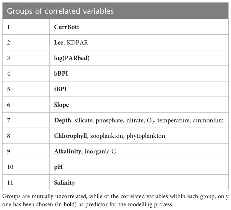
Table 2 Groups of correlated environmental variables.

2.5 Predictive model development

The random forest (RF) classification algorithm was used in this work for predictive model development. RF has recently been used for habitat suitability modelling works (Pearman et al., 2020; Jackson-Bué et al., 2022) exhibiting significant results. It is preferred against other modelling techniques because it makes no underlying assumptions of the variables’ distributions, it is robust to overfitting, it allows for non-linear interactions between the response and environmental variables (Cutler et al., 2007; Zhang et al., 2019), and it can handle existence–absence data.

The Waikato Environment for Knowledge Analysis (WEKA V3.9.6) software, developed by the University of Waikato, Hamilton, New Zealand, was used for performing RF classification on the absence–presence data to build the spatial distribution probability model of the coralligenous formations in the Greek Seas. RF is an ensemble learning method for classification, which is based on multiple decision trees, thus the forest, for the final classification of a sample based on the majority vote. Through this procedure, the major drawback of overfitting the results based on training data by a single tree is diminished using multiple trees of random variables. The major component of its decision tree is its root, which is the start of the tree and contains the number of variables used (N) out of the total summary of them (K). The formula N = log2 K + 1 is mostly used for the selection of the number of variances N that each tree will adopt. Each step added to the decision tree leads through two branches into a leaf or to a new decision section called the internal branch. The summary of the steps needed until the final decision is the depth of the tree. The number of trees used for the creation of a forest is the iterations. One of the most important features of the RF is the Gini index, which ranks variable importance based on average impurity decrease. In other words, the Gini index describes the ability of each variable to divide the data present in the root or internal branch into two separate sets in order to advance into the next branch or leaf. All the available data have been used for training the RF model, while, through trial and error, the number of trees for each forest was set to 200, and each tree included any variable with a maximum depth of 10. The performance of the model was assessed employing both n-fold and spatial block cross-validation (Valavi et al., 2019) principles, as described in Section 2.6.

After the classifier was built and its validation metrics were estimated in the Weka explorer environment, the exported serialized classifier file was applied to the predictors’ vector file of the entire region of the Greek Seas. This vector file was created by converting the resampled 100 × 100 m cell size rasters of the predictors into point vector files and merging them under a common data table in QGIS. The final classification output contained the probability distribution for both “coralligenous” and “non-coralligenous” bottom classes, assigned to the predictors’ point vector file for the Greek Seas along with each point’s coordinates. Using a suitably selected distribution threshold, as discussed in Section 2.6, a final classification map, classifying points with probabilities of occurrence over the threshold as “coralligenous”, was created, which was suitable for further geostatistical compensation and geographic representation.

2.6 Model performance assessment and probability threshold selection

The output of the spatial predictive model is a raster of probability distribution values for coralligenous formations’ occurrence. This means that areas with higher distribution values have higher probabilities of being covered by coralligenous formations. As mentioned in Section 2.5, the RF model was trained on the full mapping dataset to take advantage of the wide geographic span of our data and to produce predictions that account for the heterogeneity among different geographic regions. Model performance was initially assessed through a 10-fold cross validation, where 10 different RF models were trained, leaving each time a random 10% of the data out for evaluation. Given that our model predicts the existence of coralligenous formations in vast areas, often far away from the training data areas (as shown in Figure 1), it was really important to take into account spatial autocorrelation. The “random” split of data in the 10-fold cross validation infers high spatial autocorrelation in the process, which might inflate the model performance. This is because of the high resolution of the mapping data, leading the random data points to be similar to each other. To test the spatial consistency of the generated decision rules, the model performance was also evaluated via spatial block cross validation (see Valavi et al., 2019). According to this, instead of generating random cross-validation folds, spatially separated folds (blocks) are created, and the RF model is trained each time onefold and tested on the others. In our case, the three ecoregions were used as “blocks”, and the ability of the model to correctly predict coralligenous occurrences when trained on one (Ionian Sea, N. Aegean, or S. Aegean Seas) or another was examined. The accuracy of the above models was evaluated and compared to each other using the area under the receiver operating characteristic (ROC) curve (AUC). The ROC curve is a graph showing the performance of a classification model, expressed as the ratio between the true-positive rate and false-positive rate, at all classification (probability distribution) thresholds. The AUC value is eventually a threshold invariant model evaluation metric that indicates how well the model fits the test set data, from 0 (model worse than random predictions) to 1 (ideal model). An AUC = 0.5 indicates random predictions, and an AUC < 0.5 indicates a model that is worse than when random classes are assigned.

When the probabilistic model needs to be reduced to a binary classification model, where there are areas “with” or “without” coralligenous formations, then a probability distribution threshold (classification threshold) needs to be set and assume that positive predictions occur when the probability distribution values are higher than this threshold. An optimized threshold would be able to respect the initial observations with a reasonable trade-off between true predictions and misclassifications. Specification of this threshold is not straightforward, but it can be decided upon observing the model accuracy change when using different threshold values. For each threshold value, an error matrix and a selection of metrics should be considered, which document the deviation between predicted and observed classes of the test set, giving an estimate of the model performance. A selection of standard performance metrics was created from the error matrix. No single measure can fully describe the performance of a classification model, and Precision, Recall (or sensitivity), and F-Measure are estimated. Precision answers the question: “What proportion of positive identifications was actually correct?” Recall: “What proportion of actual positives was identified correctly?” F-Measure is the harmonic mean of Precision and Recall, so it is a more robust measure of the model’s performance. When these measures are plotted against the classification threshold values, one can decide on the optimal threshold that keeps Precision and Recall balanced without sacrificing the overall model’s accuracy, as quantified through the F-Measure (Esposito et al., 2021). Selecting a high threshold would make Precision rise, as more and more predictions would be correct, but Recall would decrease as some true observations would be neglected. A good threshold is located where the F-Measure vs. threshold curve has been stabilized close to its maximum values until Recall starts becoming lower than Precision. The lowest possible threshold within the above range has been chosen so as to retain high positive prediction populations. Predictions with probability densities over this threshold were considered positive “coralligenous” classification, forming the final test set, for which evaluation metrics have been reported. Kappa, the true skill statistic (TSS), overall accuracy (OA), and specificity evaluation metrics have also been estimated, as suggested by Zhang et al. (2019).

Finally, it is essential to know how similar the conditions in the predictions are to those found in the training data, while in areas where they differ much, predictions should not be considered trustworthy. An out-of-range check, comparing the training to the full dataset variable numeric ranges, was made to indicate areas where at least one predictor is not within the ranges of the equivalent of the training set.

2.7 Statistical treatment and presentation

Statistical analyses in the context of the present study were performed for both the observations and the model predictions. Principal component analysis (PCA) with biplot interpretation was performed with the PAST statistical software to reveal any underlying mechanisms that link specific environmental/oceanographic variables to higher probabilities of “coralligenous” encounters. Violin plots were also created in the same software to compare the value distribution of the selected variables between the areas with or without coralligenous formations and to investigate any direct classification boundaries that each one offers. The latter was performed on the predicted “coralligenous” occurrences using the classification threshold decided through the model validation process.

3 Results

3.1 Model performance, distribution thresholding, and final predictions

We prepared one ROC curve for the 10-fold cross-validation process and another three for when training the model on each spatial block (i.e., ecoregion) and evaluating the others. Figure 4A presents the comparison between these ROC curves. All models exhibited high AUCs (>0.95), except for the one trained on the N. Aegean ecoregion block (AUC = 0.79), whose performance was apparently affected by the relatively low quantity of training data located therein. Nonetheless, the spatial autocorrelation of available data has been proven high, allowing the model to perform well when trained on either the Ionian or S. Aegean block, let alone when trained on the full dataset (exhibiting AUC = 0.99).

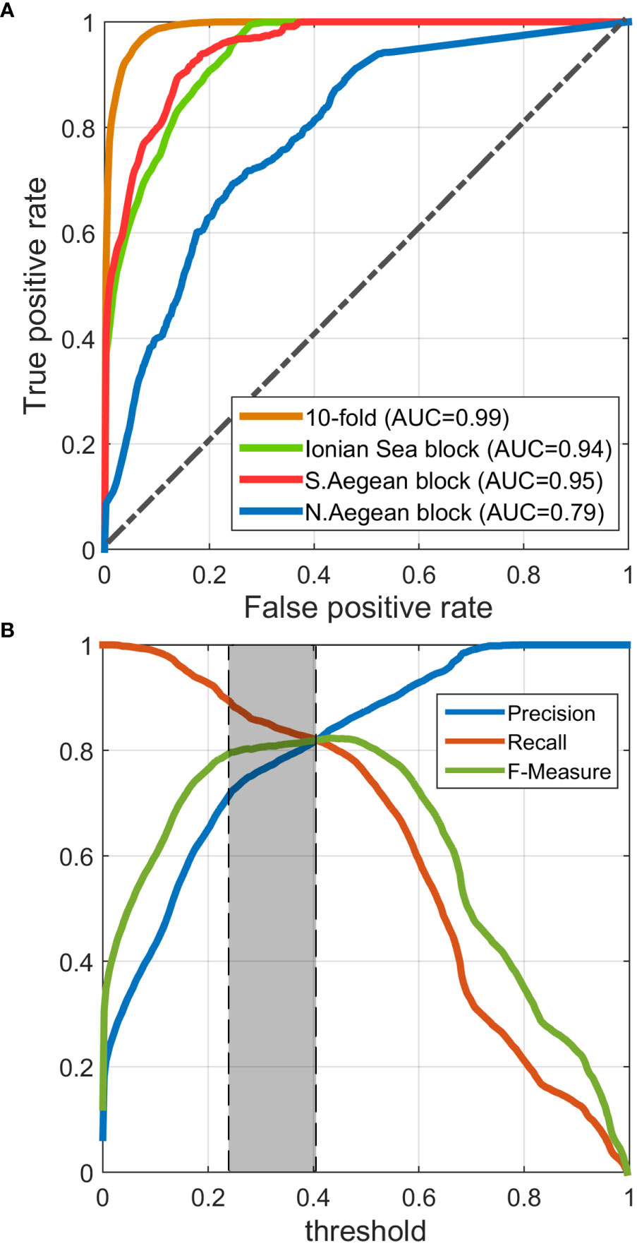
Figure 4 (A) Receiver operating characteristic (ROC) curves corresponding to the cross-validation results either on a random 10-fold of the training set or on each ecoregion. (B) Precision, Recall, and F-Measure vs. decision threshold curves, suggesting an optimized threshold between 0.23 and 0.41 (0.23 has been selected).

The reported model evaluation metrics in Table 3 correspond to the classification scheme that occurs when training the model on the full training dataset and validating it on the full dataset or either ecoregion after having selected the optimized classification threshold. As mentioned in Section 2.6, threshold selection was performed based on Precision, Recall, and F-Measure, plotted against the threshold, as illustrated in Figure 4B. This plot suggests an optimized threshold choice between 0.23 and 0.41. The minimum suggested threshold of 0.23 has eventually been selected to achieve the maximum population of positive predictions, retaining a good balance between Precision and Recall and a high F-Measure. For this threshold, all metrics indicate very good performance of the model, reaching overall accuracies between 95.89% and 98.81%, kappa values from 71.2% to 85.26%, and low false-positive rates (0.97%–3.34%), implying that the predictions meet the great majority of the observed classes, producing insignificant numbers of false predictions.

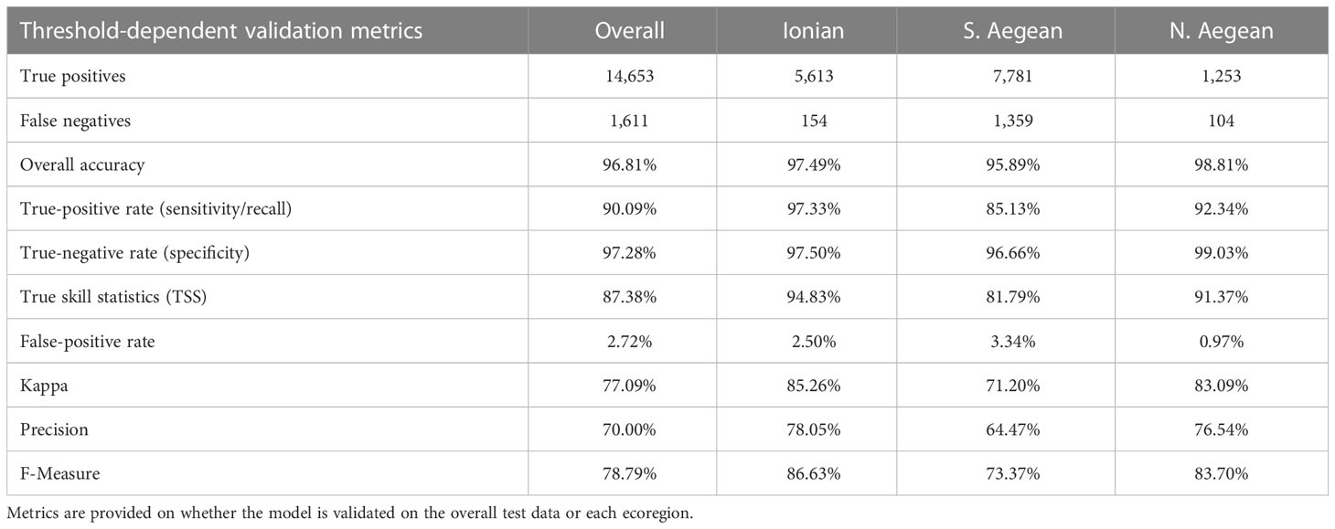
Table 3 Model validation metrics for a classification threshold equal to 0.23, as assessed through the threshold analysis in the context of the model validation process.

The spatial distribution model, showing the occurrence probabilities of coralligenous formations in the Greek Seas, is illustrated in Figure 5, in which predictions accounting for the selected classification threshold (>0.23) are indicated with red colour, while any areas where at least one predictor is not within the ranges of the equivalent in the training set are shaded out as of low reliability. A citable GeoTiff raster image of the model output has been made available in the figshare (https://figshare.com/) open data repository (https://doi.org/10.6084/m9.figshare.22276456.v2).

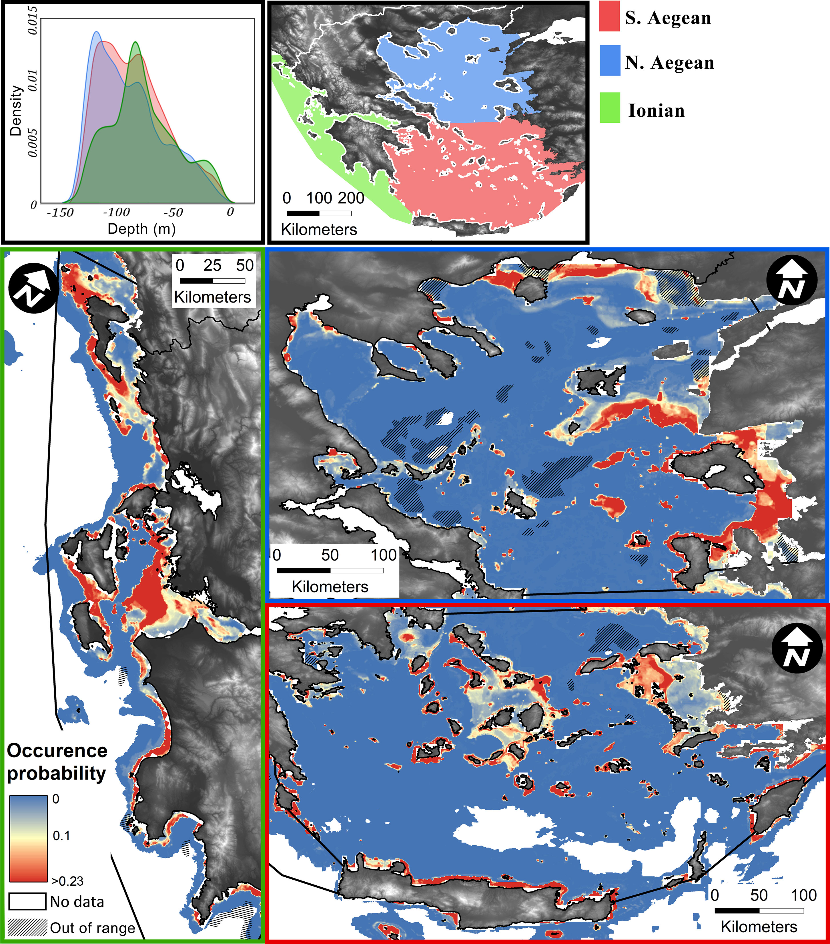
Figure 5 Predictive model spatial output presented by ecoregion (Ionian, S. Aegean, and N. Aegean). The colour scale corresponds to the probability distribution for coralligenous formations, with values over 0.23 classification threshold indicated in red colour. Areas where predictors are out of range in regard to the training set are overlayed by a linear hatch. Upper right is the water depth probability density function for areas classified as “coralligenous” per ecoregion.

3.2 Environmental variables’ importance

The Gini index coefficient estimated within the RF algorithm (Figure 6) indicated that Lee’s euphotic depth was the variable offering the highest information gain to the learning process, followed by CurrBott and PARbed with values ranging from 0.30 to 0.28. The topographic indices, depth, bBPI, fBPI, and slope exhibited intermediate index values between 0.26 and 0.24. Chlorophyll (0.21), pH (0.19), salinity (0.18), and alkalinity (0.17) offered the least information gain. The above implies that light radiation, bottom currents, and seabed morphometry seem to be the main factors controlling the spatial distribution of coralligenous formations.

Figure 6 The Gini index weighting the variables’ importance in the RF model. RF, random forest.

In Figure 1, the water depth probability density function for observations with coralligenous formations is presented per ecoregion (Ionian, S. Aegean, and N. Aegean Seas), clearly showing that they have not been detected deeper than 140 m. The same has been shown through spatial predictive modelling, as shown in the depth probability densities in Figure 5. To closely investigate which environmental variables control the spatial distribution of coralligenous formations, the model predictions have thus been narrowed to the 0–140-m depth range, and PCA has been applied to the updated predictors’ vector. A PCA biplot (Figure 7) has been created using the first two PCs, mixing PC scores with variables’ loadings in the same PC axes. Minimum volume ellipsoids enclosing 60% of the PC scores of each bottom class were also drawn to visualize the separation between “coralligenous” and “non-coralligenous” classes and to investigate which variables they are controlled by.

Figure 7 PCA biplot as applied to the model predictions narrowed to the 0–140-m depth range. Ellipses indicate 70% minimum volume ellipsoids for areas classified by the RF model (using the 0.23 threshold) as covered with coralligenous formations or not. PC scores are represented as dots with colours corresponding to bottom class and green lines to the variables’ loading vectors. PCA, principal component analysis; RF, random forest; PC, principal component.

The environmental variables that have been found, through the above analyses, to be controlling the most the spatial occurrences of coralligenous formations were further analysed to detect any distinct data thresholds separating them from areas without such formations. For this, the probability density of each “important” predictor’s values is visually compared between areas with or without coralligenous formations through violin plots, as illustrated in Figure 8.

Figure 8 Violin/box plots comparing the values distribution of the main predictors for areas classified by the RF model (using the 0.23 threshold) as “coralligenous” or “non-coralligenous”. RF, random forest.

4 Discussion

4.1 Mapped and predicted spatial patterns of coralligenous formations in the Greek Seas

In total, a mapped area of 3,197.68 km² has been archived, 6.62% (211.67 km²) of which was covered by coralligenous formations. In the 20–140 m depth range (1,051 km²), where the coralligenous formations are exclusively narrowed to, their coverage reaches 16.2% (169.94 km²). In the Ionian and S. Aegean Seas, the mapped depth distributions are similar, illustrating a mean depth of 90 m, while in N. Aegean, the mean depth is approximately 40 m (see Figure 1). However, the depth distribution of coralligenous formations, as estimated through the spatial probability modelling, indicates that there is a common distribution of depths in all ecoregions, with N. Aegean having a bimodal statistical distribution (Figure 5). The shallower mode of this corresponds to the northern parts of N. Aegean, on the coasts of Chalkidiki and Kavala-Thassos, where the Black Sea water outflow causes significantly different physicochemical properties in the water column.

The area of Greece with the most extensively mapped areas of coralligenous formations was the S. Aegean Sea. In a total of 1,455.21 km² mapped seafloor, 7.82% (113.8 km²) had coralligenous formations. The Cyclades Plateau is where the most extensive and well-formed reefs of all Greek sites were found. Significant formations were also mapped in the Kythira Elafonisos Strait (southwestern edge of the south Aegean Sea) and around Leros Island (Dodecanese, S. Aegean Sea). In the Saronic Gulf, formations were mapped in its central part and its southern border. The N. Aegean Sea was the least mapped area of the Greek Seas by LMGPO (524.36 km² where coralligenous formations were found in 4.18% (21.93 km²) of the surveyed areas. Coralligenous formations were also mapped in the Evoikos, Pagasitikos, and Toroneos Gulfs and Kavala Bay. In the N. Evoikos Gulf, the most well-formed buildups were mapped. In the Ionian Sea, a total area of 906.85 km² was mapped, and coralligenous formations were found in 75.92 km² (8.37%). In the northern part of the Ionian Sea, most of the formations were found north of Corfu Island and towards the mainland. Major formations were also mapped in the S. Ionian Sea and outer Patraikos Gulf. Formations were also mapped in the Amvrakikos Gulf, although it is a semi-enclosed, fjord-like marine environment. In the Evoikos and Amvrakikos Gulfs, there was no data coverage regarding the environmental variables, and thus, no predictive mapping has been performed there.

Model predictions honoured in great precision the observations and indicated areas where coralligenous formations are likely to have significant extents (Figure 5). In the Ionian Sea, the model projected three areas with high probabilities of coralligenous formations' existence, namely, N. Ionian (Corfu and Paxos Islands), central Ionian (outer Patraikos Gulf and Zakynthos–Kefalonia Straits), and SW Peloponnese (Kyparissiakos Gulf to Pylos). In the S. Aegean Sea, four areas exhibit high coralligenous formations’ occurrence probabilities, namely, the Cyclades Plateau, N. Crete, the Dodecanese Islands, and the Kythira–Crete strait. In the N. Aegean Sea, Kavala Bay, N. Aegean Islands (Limnos, Lesvos, and Chios), outer Thermaikos, N. Pagasitikos, and Ierissos Gulfs are likely to have extensive coralligenous formations.

The spatial patterns of coralligenous formations’ occurrence probabilities in Greece as estimated in the present work are generally similar to those in Martin et al. (2013). Some major deviations though can be detected in Lesvos and Chios (NE Aegean), between Ikaria and Kos (SE Aegean) and in S. Corfu (N. Ionian) islands, where more abundant formations are predicted in the present work, while in E Limnos (N. Aegean), no formations are predicted herein, as justified also by our field data. The validity of any of the above models could only be assessed with the acquisition of more mapping data via targeted samplings.

4.2 Suitability ranges of environmental variables

The learning process of the RF predictive model involved, through the Gini index, weighting the importance of each environmental predictor regarding the degree it aided in producing correct decisions. As shown in Figure 6, light irradiance, expressed via the Lee euphotic depth and the seabed PAR, and hydrodynamics (bottom currents) exhibited top gains in the classifier’s learning process, followed by all the topographic indices. The PCA biplot (Figure 7) explaining 57% of the data variance projected almost all predictors with high loadings in the PC1 vs. PC2 axes. Lee and salinity vectors were positively correlated to the PC scores of the coralligenous formations; alkalinity, pH, and chlorophyll vectors negatively correlated to them, while all topographic indices were orthogonal (perpendicular) to the aforementioned ones. The predictive power of the selected variables is thus proven significant, given that the predictions’ scores exhibited significant separation between “coralligenous” and “non-coralligenous” classes in the PC1 vs. PC2 space, especially when combining at least two variables orthogonal to each other PC loading, forming well-separated prediction classes in the Euclidean space.

Regarding light attenuation, the violin plots of Lee and PARbed in the 0–140 m depth range (Figure 8) indicate that coralligenous formations are expected where the euphotic depth is high (greater absorption of light irradiance in the water column) and the PAR on the seafloor is moderate. This is attributed to the sciaphilic nature of the coralligenous algae. In this study, coralligenous formations have been found and predicted in areas where the irradiance reaching the seafloor (PARbed) was between 0.005% and 3% of the surface one, which is also supported by Ballesteros (2006). Moreover, the violin plots indicate that the majority of coralligenous formations are found where Lee is in a narrow range between 65 and 68 m and the depth is below −70 m. Lee euphotic depth is derived as the depth in the water column that PAR is 1% of its surface value; thus, the above ranges imply that formations are mostly found where PAR is even lower.

Bottom currents (CurrBott), although not exhibiting high loadings in the PC1 vs. PC2 biplot (it had greater loadings in PC4), nor any distinctive range thresholds can be drawn in the violin plots (Figure 8), have been attributed to one of the highest importance scores due to the Gini index. The importance of hydrodynamics in coralligenous formation development has previously been reported in the literature. Unattached corals, like maerl and rhodoliths, are subject to mechanical abrasion under strong currents (Basso et al., 2009). Water movement, to some level, however, is crucial, as it enables oxygen circulation and keeps their surface clean (Larkum et al., 2003) while simultaneously protecting them from poisoning through water stagnation (Basso, 1998; Nelson et al., 2012). Moreover, as bottom currents are the means for sediment transport, they are controlling sedimentation rates on the seafloor. Since coralligenous formations have very slow growth rates (Ballesteros, 2006; Caragnano et al., 2016), areas where the sedimentation rate is higher than the growth rate are not suitable for their development (Basso, 1998; Dethier and Steneck, 2001; Foster, 2001; Riul et al., 2009; Villas-Bôas et al., 2014). Thus, coralligenous formations build in a specific range of bottom current speeds, as they require currents strong enough to mix the seawater but not that strong as to detach the thalli of the formations from the seafloor. More closely examining bottom current speed distribution in the violin plots, no formation has been in areas with less than 0.5 cm/s water speeds, while few develop in areas with over 3 cm/s of water speed.

Topographic variables have been given relatively high importance in the model development, as expressed through the Gini index, and they also exhibited high PC loadings in the PCA biplot. Especially slope, bBPI, and fBPI exhibit considerably different value distributions in areas with coralligenous formations than in areas without ones (Figure 8), showcasing the importance of topographic indices for the suitability modelling of coralligenous formations in the Mediterranean. Buildups seem to develop in areas with exclusively positive bBPI values, i.e., on large-scale ridges and mounds, avoiding flat basins and valleys. The same is supported by fBPI, which exhibits 25th–75th percentiles in the −1 to 61 range for areas classified as “coralligenous” and −3 to 7 for “non-coralligenous”, implying that buildups developed on finer-scale bathymetric ridges and mounds and their lower slopes. Likewise, coralligenous formations seem to avoid slopes close to 0 and develop on areas with slopes in the range of 1° to 5° and mainly on mild slopes (mean of 1.5°). The above is in agreement that coralligenous formations (especially reefs) are known to develop in sub-cropping or out-cropping areas (Got and Laubier, 1968; Laborel, 1987; Georgiadis et al., 2009; Dimas et al., 2022), which inherently form ridges and mounds on the seafloor, including the coastal slopes where the bedrock is also sub- or out-cropping. This finding is an addition to the previous knowledge. For instance, in Georgiadis et al. (2009) and Martin et al. (2013), the Cyclades Plateau was considered to have high occurrence probabilities of coralligenous formations throughout its 70–100 m bathymetric range. This was due to the insufficient presence–absence data used for drawing assumptions or developing predictive models, making it difficult to draw the dependency between coralligenous formations and local seabed morphology. In the present study, the spatial extents of coralligenous formations in the Cyclades Plateau are predicted on peripheral to the Plateau large-scale ridges and upper slopes, exactly validating the plethora of observations that have been archived in the area.

Both salinity and alkalinity values in areas with coralligenous formations exhibited very distinctive distributions in the violin plots of Figure 8. Their loading vectors were also significant in the PCA biplot (Figure 7), implying a preference for coralligenous formations to develop in bottoms with high salinity and low alkalinity. More specifically, the “coralligenous” class shows a clear preference for the upper range of the modelled bottom salinity values, with its 25th–75th percentiles being 39.1–39.2 PSU out of a total variation in the 0–140 m depth range of the Greek Seas of 37.8–39.3 PSU. Alkalinity exhibited a clear threshold at 2.72 mmol/m³, with coralligenous formations appearing to occur in the narrow 2.71–2.72 mmol/m³ range, and without ones almost exclusively over it.

pH distribution, although obtaining middle-to-low values (more acidic), is in the narrow range of 8.106–8.116 for seafloors classified as “coralligenous”, in comparison to the 8.11–8.146 range for “non-coralligenous. The same occurs for chlorophyll, with coralligenous formations preferring moderate values, between 0.086 and 0.153 mg/m³ out of the 0.11–0.19 mg/m³ total range in the 0–140 m depth range. Even though chlorophyll and pH value distribution did not show any clear separatory thresholds between areas with and without coralligenous formations, they seem to have been more important than salinity and alkalinity in the classification process according to the Gini index (Figure 6), while they also take high PC loading in the PCA biplot (Figure 7). This is because the formations mapped on the Thracian coastal areas on the N end of N. Aegean are directly influenced by the exchanges with the high pH and chlorophyll Black Sea water masses, so the RF model ranked them high in an effort to correctly classify them in space. Finally, although the bottom temperature has not been selected as a model predictor (being linearly correlated to depth), it is an important environmental variable, and as such, its distribution is examined. It exhibits similar median values for areas with or without coralligenous formations (16.8°C), not forming any sharp threshold between them. Nevertheless, coralligenous formations show preference in the narrow range between 16°C and 17°C (distribution peak), while its main distribution in the Greek shallow bottoms (depth < 140 m) is between 15°C and 18°C.

4.3 Coralligenous formation growth rates and paleogeographic implications

There is a discussion about whether Mediterranean coralligenous formations in deep waters (>50 m) are still active or not. As discussed in Ballesteros (2006), the growth rate in formations found in the NW Mediterranean, at depths between 10 and 60 m, presented a great variety between 0.006 and 0.83 mm/year, depending on the depth they were found and the geologic period they were formed. Two growth rates were distinguished: a) higher growth rate (0.11 to 0.42 mm/year), placed in relatively shallow areas of 10 to 35 m, and b) low growth rates, reaching 0 in the 50–60 m depth. The latter corresponds to formations developed between 8k and 5k years BP, a geologic period when they have reached their maximum growth rate, estimated at approximately 0.20 to 0.83 mm/year.

Our field data show a maximum coverage of coralligenous formations between 63 and 110 m depth (mean depth of 90 m). If we assume a water depth of 35 m for maximum coralligenous algae growth (Ballesteros, 2006) and based on the global eustatic sea level curves (Lambeck et al., 2014), then those coralligenous formations should have been developed approximately 13 and 9 ka BP. This interval corresponds to a transitional period between the Last Glacial low sea-level stand and the Holocene high sea-level stand. Sedimentological studies have shown that in this period, the seafloor in the studied area started to experience more active bottom currents, together with the sea level rise (Tripsanas et al., 2015) and more eutrophicated conditions linked to increases in precipitation, high levels of marine productivity, and strengthening of water-column stratification (Rohling et al., 2015).

However, in the Thracian Sea (N end of N. Aegean), in Amvrakikos Gulf and N Evoikos Gulf, the shallowest coralligenous formations have been detected in depths of between 20 and 50 m. These areas are characterized by very turbid waters and shallow euphotic depths, as they are affected by river outflows and the Black Sea water mass exchanges, or they are semi-enclosed gulfs with high chlorophyll productions, likely forming suitable conditions for coralligenous algae (known to be sciaphilic). Whether these formations are active or not today and, if they are, which is the trigger mechanism for their growth, especially in the deeper waters, are high-priority research topics that have not yet been studied.

5 Conclusions

Although coralligenous formations are EU-priority habitats and among the most crucial marine habitats in the Mediterranean Sea, their spatial distribution is still majorly unknown. Found in wide geographic extend and depth ranges (10–140 m), great effort and time are needed by marine researchers to completely map them using hydroacoustic and visual census systems. In the Greek Seas, the available data about these formations are sparse and mainly from in situ presence-only opportunistic observations, having left great gaps and uncertainties about their true distribution. The present work amalgamates some of the most broad-scale hydroacoustic datasets available in Greece and constructs the first presence–absence geodatabase of coralligenous formations in its Seas. Based on it, a predictive distribution model has been developed, using as predictors a variety of key environmental seafloor variables, from depth morphometry derivatives and hydrodynamics to light irradiance and physicochemical seawater properties. The adequacy and the substantial geographic distribution of the presence–absence data fed in the model’s training process, along with the relevance of the variables used as predictors, generated a reliable predictive map of their distribution in the Greek Seas. Through this, commenting on the geographic distribution of the formations and implications about the suitability of the predictors for controlling their development were made. Light irradiance and seafloor currents, as already reported in past bibliographic resources, were found to be among the most important environmental variables. Bathymetric indices were also proven powerful descriptors, with coralligenous formations showing clear preference in elevated areas, like ridges and mounds, being totally absent in large-scale depressions, like valleys and basins, implying a strong relation of their development to geomorphology. Questions still arise about whether and to what extent these formations are still building up, especially in their deeper margins, or whether they are paleontological remnants. In any case, they are one of the most important biodiversity hotspots in the Mediterranean, and endeavours such as the present work are stepping stones for implementing successful ecological management and spatial planning activities.

Data availability statement

The original contributions presented in the study are included in the article/Supplementary Material. Further inquiries can be directed to the corresponding authors.

Author contributions

Conceptualization: EF, GP, CK, GF, and MG. Methodology: EF and XD. Software: EF. Validation: EF, XD, and GP. Data retrieval/digitization/archiving: VG, XD, and EF. Data curation: EF, XD, and VG. Statistical treatment: EF. Writing—original draft: EF and XD. Review and editing: GP and MG. Visualization: EF and XD. Supervision: GP. All authors contributed to the article and approved the submitted version.

Funding

This research is co-financed by Greece and the European Union (European Social Fund—ESF) through the Operational Programme “Human Resources Development, Education and Lifelong Learning” in the context of the project “Reinforcement of Postdoctoral Researchers—2nd Cycle” (MIS-5033021), implemented by the State Scholarships Foundation (IKY). Data acquisition and interpretation are a cumulative effort of more than 34 unclassified academic and commercial projects of Oceanus-Lab, spanning 31 years of research. The publication fees of this manuscript have been financed by the Research Council of the University of Patras.

Acknowledgments

We would like to thank all diachronic members of Oceanus-Lab, Geology Department, University of Patras, Greece (https://oceanus-lab.upatras.gr/).

Conflict of interest

The authors declare that the research was conducted in the absence of any commercial or financial relationships that could be construed as a potential conflict of interest.

Publisher’s note

All claims expressed in this article are solely those of the authors and do not necessarily represent those of their affiliated organizations, or those of the publisher, the editors and the reviewers. Any product that may be evaluated in this article, or claim that may be made by its manufacturer, is not guaranteed or endorsed by the publisher.

Supplementary material

The Supplementary Material for this article can be found online at: https://www.frontiersin.org/articles/10.3389/fmars.2023.1117919/full#supplementary-material

References

Ballesteros E. (2006). Mediterranean Coralligenous assemblages: a synthesis of present knowledge. Oceanogr. Mar. Biol. 44, 123–195. doi: 10.1201/9781420006391-7
Bargain A., Foglini F., Pairaud I., Bonaldo D., Carniel S., Angeletti L., et al. (2018). Predictive habitat modeling in two Mediterranean canyons including hydrodynamic variables. Prog. Oceanogr. 169, 151–168. doi: 10.1016/j.pocean.2018.02.015
Bartlett C. Y., Manua C., Cinner J., Sutton S., Jimmy R., South R., et al. (2009). Comparison of outcomes of permanently closed and periodically harvested coral reef reserves. Conserv. Biol. 23, 1475–1484. doi: 10.1111/j.1523-1739.2009.01293.x
Basso D. (1998). Deep rhodolith distribution in the pontian islands, Italy: a model for the paleoecology of a temperate sea. Palaeogeogr. Palaeoclimatol. Palaeoecol. 137, 173–187. doi: 10.1016/S0031-0182(97)00099-0
Basso D., Nalin R., Nelson C. S. (2009). Shallow-water sporolithon rhodoliths from north island (New Zealand). Palaios 24, 92–103. doi: 10.2110/palo.2008.p08-048r
Blondel P., Huvenne V., Huhnerbach V. (2006). “Multi-frequency acoustics of deep-water coral habitats and textural characterisation,” in Proceedings of the Eighth European Conference on Underwater Acoustics, (8th ECUA), Carvoeiro, Portugal, 12-15 June. (Carvoeiro, Portugal: ECUA Secretariat)
Bonacorsi M., Pergent-Martini C., Clabaut P., Pergent G. (2012). Coralligenous “atolls”: discovery of a new morphotype in the Western Mediterranean Sea. C R Biol. 335, 668–672. doi: 10.1016/j.crvi.2012.10.005
Brown C. J., Smith S. J., Lawton P., Anderson J. T. (2011). Benthic habitat mapping: a review of progress towards improved understanding of the spatial ecology of the seafloor using acoustic techniques. Estuar. Coast. Shelf Sci. 92, 502–520. doi: 10.1016/j.ecss.2011.02.007
Caragnano A., Basso D., Rodondi G. (2016). Growth rates and ecology of coralline rhodoliths from the ras ghamila back reef lagoon, red Sea. Mar. Ecol. 37, 713–726. doi: 10.1111/maec.12371
Cogan C. B., Todd B. J., Lawton P., Noji T. T. (2009). The role of marine habitat mapping in ecosystem-based management. ICES J. Mar. Sci. 66 (9), 2033–2042. doi: 10.1093/icesjms/fsp214
Coll M., Piroddi C., Albouy C., Ben Rais Lasram F., Cheung W. W. L., Christensen V., et al. (2012). The Mediterranean Sea under siege: spatial overlap between marine biodiversity, cumulative threats and marine reserves. Global Ecol. Biogeogr. 21, 465–480. doi: 10.1111/j.1466-8238.2011.00697.x
Collier J. S., Brown C. J. (2005). Correlation of sidescan backscatter with grain size distribution of surficial seabed sediments. Mar. Geol. 214, 431–449. doi: 10.1016/j.margeo.2004.11.011
Collier J. S., Humber S. R. (2007). Time-lapse side-scan sonar imaging of bleached coral reefs: a case study from the Seychelles. Remote Sens. Environ. 108 (4), 339–356. doi: 10.1016/j.rse.2006.11.029
Cutler D. R., Edwards T. C. Jr., Beard K. H., Cutler A., Hess K. T., Gibson J., et al. (2007). Random forests for classification in ecology. Ecology 88, 2783–2792. doi: 10.1890/07-0539.1
Davies A. J., Guinotte J. M. (2011). Global habitat suitability for framework-forming cold-water corals. PloS One 6, e18483. doi: 10.1371/journal.pone.0018483
Davies A. J., Wisshak M., Orr J. C., Murray Roberts J. (2008). Predicting suitable habitat for the cold-water coral lophelia pertusa (Scleractinia). Deep Sea Res. Part I: Oceanographic Res. Pap. 55, 1048–1062. doi: 10.1016/j.dsr.2008.04.010
De Falco G., Conforti A., Brambilla W., Budillon F., Ceccherelli G., De Luca M., et al. (2022). Coralligenous banks along the western and northern continental shelf of Sardinia island (Mediterranean Sea). J. Maps. 18, 200–209. doi: 10.1080/17445647.2021.2020179
Dethier M. N., Steneck R. S. (2001). Growth and persistence of diverse intertidal crusts: survival of the slow in a fast-paced world. Mar. Ecol. Prog. Ser. 223, 89–100. doi: 10.3354/meps223089
Di Maida G., Tomasello A., Luzzu F., Scannavino A., Pirrotta M., Orestano C., et al. (2011). Discriminating between posidonia oceanica meadows and sand substratum using multibeam sonar. ICES J. Mar. Sci. 68, 12–19. doi: 10.1093/icesjms/fsq130
Dimas X., Fakiris E., Christodoulou D., Georgiou N., Geraga M., Papathanasiou V., et al. (2022). Marine priority habitat mapping in a Mediterranean conservation area (Gyaros, south Aegean) through multi-platform marine remote sensing techniques. Front. Mar. Sci. 9. doi: 10.3389/fmars.2022.953462
Esposito C., Landrum G. A., Schneider N., Stiefl N., Riniker S. (2021). GHOST: adjusting the decision threshold to handle imbalanced data in machine learning. J. Chem. Inf. Modeling 61 (6), 1549–9596. doi: 10.1021/acs.jcim.1c00160
Fakiris E. (2012). Developing computational tools for the processing and analysis of marine geophysical data. applications to Ionian Sea, Aegean Sea and patraikos gulf, Greece (Greece: University of Patras). PhD thesis.
Fakiris E., Blondel P., Papatheodorou G., Christodoulou D., Dimas X., Georgiou N., et al. (2019). Multi-frequency, multi-sonar mapping of shallow habitats–efficacy and management implications in the national marine park of zakynthos, Greece. Remote Sens. (Basel) 11, 461. doi: 10.3390/rs11040461
Fakiris E., Papatheodorou G. (2012). Quantification of regions of interest in swath sonar backscatter images using grey-level and shape geometry descriptors: the TargAn software. Mar. Geophys. Res. 2, 169–183. doi: 10.1007/S11001-012-9153-5
Fakiris E., Zoura D., Ramfos A., Spinos E., Georgiou N., Ferentinos G., et al. (2018). Object-based classification of sub-bottom profiling data for benthic habitat mapping. comparison with sidescan and RoxAnn in a Greek shallow-water habitat. Estuar. Coast. Shelf Sci. 208, 219–234. doi: 10.1016/j.ecss.2018.04.028
Foster-Smith B., Connor D., Davies J. (2008). “MESH guide: what is habitat mapping?,” in MESH guide to habitat mapping: a synopsis. Eds. Davies J., Young S. (Peterborough: Joint Nature Conservation Committee), 11–24.
Foster M. S. (2001). Rhodoliths: Between rocks and soft places. J Phycol 37, 659–667. doi: 10.1046/j.1529-8817.2001.00195.x
Franklin J., Miller J. I. (2010). Mapping species distributions (Cambridge: Cambridge University Press). doi: 10.1017/CBO9780511810602
Georgiadis M., Papatheodorou G., Tzanatos E., Geraga M., Ramfos A., Koutsikopoulos C., et al. (2009). Coralligène formations in the eastern Mediterranean Sea: morphology, distribution, mapping and relation to fisheries in the southern Aegean Sea (Greece) based on high-resolution acoustics. J. Exp. Mar. Biol. Ecol. 368, 44–58. doi: 10.1016/j.jembe.2008.10.001
Geraga M., Papatheodorou G., Agouridis C., Kaberi H., Iatrou M., Christodoulou D., et al. (2017). Palaeoenvironmental implications of a marine geoarchaeological survey conducted in the SW argosaronic gulf, Greece. J. Archaeol. Sci. Rep. 12, 805–818. doi: 10.1016/j.jasrep.2016.08.004
Giakoumi S., Sini M., Gerovasileiou V., Mazor T., Beher J., Possingham H. P., et al. (2013). Ecoregion-based conservation planning in the Mediterranean: dealing with Large-scale heterogeneity. PloS One 8. doi: 10.1371/journal.pone.0076449
Got H., Laubier L. (1968). Prospection sysmique au large des albères: nature du substrat originel du coralligène. Vie Milieu 19, 9–16.
Guisan A., Zimmermann N. E. (2000). Predictive habitat distribution models in ecology. Ecol. Modell 135, 147–186. doi: 10.1016/S0304-3800(00)00354-9
Hamer Ø., Harper D. A. T., Ryan P. D. (2001). PAST: PAleontological STatistics software package for education and data analysis. Palaeontologia Electronica 4 (1), 9.
Ingrassia M., Martorelli E., Sañé E., Falese F. G., Bosman A., Bonifazi A., et al. (2019). Coralline algae on hard and soft substrata of a temperate mixed siliciclastic-carbonatic platform: sensitive assemblages in the zannone area (western pontine archipelago; tyrrhenian Sea). Mar. Environ. Res. 147, 1–12. doi: 10.1016/j.marenvres.2019.03.009
Innangi S., Tonielli R., Romagnoli C., Budillon F., Di Martino G., Innangi M., et al. (2019). Seabed mapping in the pelagie islands marine protected area (Sicily channel, southern Mediterranean) using remote sensing object based image analysis (RSOBIA). Mar. Geophys. Res. 40, 333–355. doi: 10.1007/s11001-018-9371-6
Jackson-Bué T., Williams G. J., Whitton T. A., Roberts M. J., Brown A. G., Amir H., et al. (2022). Seabed morphology and bed shear stress predict temperate reef habitats in a high energy marine region. Estuar. Coast. Shelf Sci. 274, 107934. doi: 10.1016/j.ecss.2022.107934
Laborel J. (1987). Marine biogenic constructions in the mediterranean. a review. Trav. Sci. du Parc Natl. Port-Cros., 281–310. doi: 10.1007/978-94-009-4215-8_10
Lacharité M., Brown C. J., Gazzola V. (2018). Multisource multibeam backscatter data: developing a strategy for the production of benthic habitat maps using semi-automated seafloor classification methods. Mar. Geophys. Res. 39, 307–322. doi: 10.1007/s11001-017-9331-6
Lambeck K., Rouby H., Purcell A., Sun Y., Sambridge M. (2014). Sea Level and global ice volumes from the last glacial maximum to the holocene. proc. Natl. Acad. Sci. 111, 15296–15303. doi: 10.1073/pnas.1411762111
Larkum A. W. D., Koch E. M. W., Kühl M. (2003). Diffusive boundary layers and photosynthesis of the epilithic algal community of coral reefs. Mar. Biol. 142, 1073–1082. doi: 10.1007/s00227-003-1022-y
Le Bas T. P., Huvenne V. A. I. (2009). Acquisition and processing of backscatter data for habitat mapping - comparison of multibeam and sidescan systems. Appl. Acous. 70, 1248–1257. doi: 10.1016/j.apacoust.2008.07.010
Lee Z. P., Weidemann A., Kindle J., Arnone R., Carder K. L., Davis C. (2007). Euphotic zone depth: its derivation and implication to ocean-color remote sensing. J. Geophys. Res. Ocean. 112. doi: 10.1029/2006JC003802
Lundblad E. R., Wright D. J., Miller J., Larkin E. M., Rinehart R., Naar D. F., et al. (2006). A benthic terrain classification scheme for American Samoa. Mar. Geod. 29, 89–111. doi: 10.1080/01490410600738021
Marchese F., Bracchi V. A., Lisi G., Basso D., Corselli C., Savini A. (2020). Assessing fine-scale distribution and volume of Mediterranean algal reefs through terrain analysis of multibeam bathymetric data. a case study in the southern Adriatic continental shelf. Water (Basel) 12, 157. doi: 10.3390/w12010157
Martin S., Charnoz A., Gattuso J. P. (2013). Photosynthesis, respiration and calcification in the Mediterranean crustose coralline alga lithophyllum cabiochae (Corallinales, rhodophyta). Eur. J. Phycol. 48, 163–172. doi: 10.1080/09670262.2013.786790
Martin C. S., Giannoulaki M., De Leo F., Scardi M., Salomidi M., Knitweiss L., et al. (2014). Coralligenous and maërl habitats: predictive modelling to identify their spatial distributions across the mediterranean sea. Sci. Rep. 4, 1–9. doi: 10.1038/srep05073
Micallef A., Le T. P., Huvenne V. A. I. I., Blondel P., Deidun A., Veit H., et al. (2012). A multi-method approach for benthic habitat mapping of shallow coastal areas with high-resolution multibeam data. Cont. Shelf Res., 39–40. doi: 10.1016/j.csr.2012.03.008
NASA Goddard Space Flight Center, Ocean Ecology Laboratory, Ocean Biology Processing Group (2022). Medium resolution imaging spectrometer (MERIS) ZLEE data (Greenbelt, MD, USA: Reprocessing. NASA OB.DAAC). doi: 10.5067/ENVISAT/MERIS/L3B/ZLEE/2022
Nelson W. A., Neill K., Farr T., Barr N., D’Archino R., Miller S., et al. (2012) Rhodolith beds in northern new Zealand: characterisation of associated biodiversity and vulnerability to environmental stressors. Available at: http://fs.fish.govt.nz/Doc/23064/AEBR_99.pdf.ashx.
Papatheodorou G., Avramidis P., Fakiris E., Christodoulou D., Kontopoulos N. (2012). Bed diversity in the shallow water environment of pappas lagoon in Greece. Int. J. Sediment Res. 27, 1–17. doi: 10.1016/S1001-6279(12)60012-2
Panayotidis P., Papathanasiou V., Gerakaris V., Fakiris E., Orfanidis S., Papatheodorou G., et al. (2022). Seagrass meadows in the Greek Seas: presence, abundance and spatial distribution. Botanica Marina 65, 289–299. doi: 10.1515/bot-2022-0011
Pearman T. R. R., Robert K., Callaway A., Hall R., Iacono C., Huvenne V. A. I. (2020). Improving the predictive capability of benthic species distribution models by incorporating oceanographic data – towards holistic ecological modelling of a submarine canyon. Prog. Oceanogr. 184, 102338. doi: 10.1016/j.pocean.2020.102338
Pérès J., Picard J. (1951). Notes sur les fonds coralligènes de la région de marseille. Arch. Zool. Expérimentale Générale 88, 24–38.
Pierdomenico M., Bonifazi A., Argenti L., Ingrassia M., Casalbore D., Aguzzi L., et al. (2021). Geomorphological characterization, spatial distribution and environmental status assessment of coralligenous reefs along the latium continental shelf. Ecol. Indic. 131, 108219. doi: 10.1016/j.ecolind.2021.108219
Prampolini M., Angeletti L., Castellan G., Grande V., Le Bas T., Taviani M., et al. (2021). Benthic habitat map of the southern adriatic sea (Mediterranean sea) from object-based image analysis of multi-source acoustic backscatter data. Remote Sens. (Basel). 13. doi: 10.3390/rs13152913
Riul P., Lacouth P., Pagliosa P. R., Christoffersen M. L., Horta P. A. (2009). Rhodolith beds at the easternmost extreme of south America: community structure of an endangered environment. Aquat. Bot. 90, 315–320. doi: 10.1016/j.aquabot.2008.12.002
Roberts J. M., Brown C. J., Long D., Bates C. R. (2005). Acoustic mapping using a multibeam echosounder reveals cold-water coral reefs and surrounding habitats. Coral Reefs 24 (4), 654–669. doi: 10.1007/s00338-005-0049-6
Rocha G. A., Bastos A. C., Amado-Filho G. M., Boni G. C., Moura R. L., Oliveira N. (2020). Heterogeneity of rhodolith beds expressed in backscatter data. Mar. Geol. 423, 106136. doi: 10.1016/j.margeo.2020.106136
Rohling E. J., Marino G., Grant K. M. (2015). Mediterranean Climate and oceanography, and the periodic development of anoxic events (sapropels). Earth-Sci. Rev. 143, 62–97. doi: 10.1016/j.earscirev.2015.01.008
Romagnoli B., Grasselli F., Costantini F., Abbiati M., Romagnoli C., Innangi S., et al. (2021). Evaluating the distribution of priority benthic habitats through a remotely operated vehicle to support conservation measures off linosa island (Sicily channel, Mediterranean Sea). Aquat. Conserv. 31, 1686–1699. doi: 10.1002/aqc.3554
Sañé E., Ingrassia M., Chiocci F. L., Argenti L., Martorelli E. (2021). Characterization of rhodolith beds-related backscatter facies from the western pontine archipelago (Mediterranean Sea). Mar. Environ. Res. 169. doi: 10.1016/j.marenvres.2021.105339
Sini M., Katsanevakis S., Koukourouvli N., Gerovasileiou V., Dailianis T., Buhl-Mortensen L., et al. (2017). Assembling ecological pieces to reconstruct the conservation puzzle of the Aegean Sea. Front. Mar. Sci. 4. doi: 10.3389/fmars.2017.00347
Tittensor D. P., Baco A. R., Brewin P. E., Clark M. R., Consalvey M., Hall-Spencer J., et al. (2009). Predicting global habitat suitability for stony corals on seamounts. J. Biogeogr. 36, 1111–1128. doi: 10.1111/j.1365-2699.2008.02062.x
Tripsanas E. K., Panagiotopoulos I. P., Lykousis V., Morfis I., Karageorgis A. P., Anastasakis G., et al. (2015). Late quaternary bottom-current activity in the south Aegean Sea reflecting climate-driven dense-water production. Mar. Geol. 375, 99–119. doi: 10.1016/j.margeo.2015.12.007
Tyberghein L., Verbruggen H., Pauly K., Troupin C., Mineur F., de Clerck O. (2012). Bio-ORACLE: a global environmental dataset for marine species distribution modelling. Global Ecol. Biogeogr. 21, 272–281. doi: 10.1111/j.1466-8238.2011.00656.x
Valavi R., Elith J., Lahoz-Monfort J. J., Guillera-Arroita G. (2019). 'blockCV: an r package for generating spatially or environmentally separated folds for k-fold cross-validation of species distribution models. Methods Ecol. Evol. 10 (2), 225–232. doi: 10.1111/2041-210X.13107
Villas-Bôas A. B., De Souza Tâmega F. T., Andrade M., Coutinho R., De Oliveira Figueiredo M. A. (2014). Experimental effects of sediment burial and light attenuation on two coralline algae of a deep water rhodolith bed in Rio de Janeiro, Brazil. Cryptogam. Algol. 35, 67–76. doi: 10.7872/crya.v35.iss1.2014.67
Walbridge S., Slocum N., Pobuda M., Wright D. (2018). ). unified geomorphological analysis workflows with benthic terrain modeler. Geosciences 8, 94. doi: 10.3390/geosciences8030094
Weiss A. D. (2001). “Topographic position and landforms analysis,” in Poster Present. ESRI User Conf, San Diego, CA, USA.
Keywords: predictive distribution modelling, habitat mapping, bioconstructions, Mediterranean, sidescan sonar
Citation: Fakiris E, Dimas X, Giannakopoulos V, Geraga M, Koutsikopoulos C, Ferentinos G and Papatheodorou G (2023) Improved predictive modelling of coralligenous formations in the Greek Seas incorporating large-scale, presence–absence, hydroacoustic data and oceanographic variables. Front. Mar. Sci. 10:1117919. doi: 10.3389/fmars.2023.1117919
Received: 07 December 2022; Accepted: 01 June 2023;
Published: 28 June 2023.
Edited by:
Nina Yasuda, The University of Tokyo, JapanReviewed by:
Dimitris Poursanidis, terrasolutions marine environment research, GreeceElena Couce, Centre for Environment, Fisheries and Aquaculture Science (CEFAS), United Kingdom
Copyright © 2023 Fakiris, Dimas, Giannakopoulos, Geraga, Koutsikopoulos, Ferentinos and Papatheodorou. This is an open-access article distributed under the terms of the Creative Commons Attribution License (CC BY). The use, distribution or reproduction in other forums is permitted, provided the original author(s) and the copyright owner(s) are credited and that the original publication in this journal is cited, in accordance with accepted academic practice. No use, distribution or reproduction is permitted which does not comply with these terms.
*Correspondence: George Papatheodorou, gpapathe@upatras.gr