Article

Analysis of Caprock Tightness for CO2 Enhanced Oil Recovery and Sequestration: Case Study of a Depleted Oil and Gas Reservoir in Dolomite, Poland

by
Małgorzata Słota-Valim
*,
Andrzej Gołąbek
,
Wiesław Szott
and
Krzysztof Sowiżdżał
Department of Geology and Geochemistry, Oil and Gas Institute, National Research Institute, 25A Lubicz Str., 31-503 Krakόw, Poland
*
Author to whom correspondence should be addressed.
Energies 2021, 14(11), 3065; https://doi.org/10.3390/en14113065
Submission received: 21 April 2021 / Revised: 13 May 2021 / Accepted: 20 May 2021 / Published: 25 May 2021
(This article belongs to the Special Issue Forecasting CO2 Sequestration with Enhanced Oil Recovery)

Abstract

:
This study addresses the problem of geological structure tightness for the purposes of enhanced oil recovery with CO2 sequestration. For the first time in the history of Polish geological survey the advanced methods, practical assumptions, and quantitative results of detailed simulations were applied to study the geological structure of a domestic oil reservoir as a potential candidate for a combined enhanced oil recovery and CO2 sequestration project. An analysis of the structure sequestration capacity and its tightness was performed using numerical methods that combined geomechanical and reservoir fluid flow modelling with a standard two-way coupling procedure. By applying the correlation between the geomechanical state and transport properties of the caprock, threshold pressure variations were determined to be a key factor affecting the sealing properties of the reservoir–caprock boundary. In addition to the estimation of the sequestration capacity of the structure, the process of CO2 leakage from the reservoir to the caprock was simulated for scenarios exceeding the threshold pressure limit of the reservoir–caprock boundary. The long-term simulations resulted in a comprehensive assessment of the total amount of CO2 leakage as a function of time and the leaked CO2 distribution within the caprock.

1. Introduction

Because CO2 emissions are an increasing problem, many strategies have been developed to reduce its emissions to the atmosphere, including mineralisation [1,2], CO2 storage at the bottom of the oceans [3], accelerated weathering [4,5], and subsurface geological storage [6]. Carbon dioxide capture at the source, followed by its long-term storage in exploited hydrocarbon reservoirs, is one of the most practical ways to reduce the CO2 concentration in the atmosphere.
Reservoir structures suitable for geological CO2 storage are most frequently water-bearing formations, depleted hydrocarbon deposits, or unminable methane-rich coal seams.
Geological formations that are selected for CO2 storage must meet the appropriate criteria related to the minimum and maximum depth of the structure. The reservoir rock parameters, including thickness, permeability, porosity, and fracture characteristics, are also critical. However, the most important criterion is the sealing quality of the rock, that is, the overburden’s integrity and thickness play key roles in assessing the safety of long-term CO2 geological storage.
Most of these criteria are met for depleted oil and gas fields because hydrocarbon production from oil and gas fields implies favourable reservoir properties, including porosity, permeability, and reservoir thickness [7].
During the geological storage of CO2, most of the injected CO2 remains in the free (liquid, gas, or supercritical) phase. This phase poses the greatest threat to the seal integrity. Under reservoir conditions, which are at elevated pressures and high temperatures, CO2 occurs in a dense gas phase, yet its density is lower than that of the formation water. Driven by the buoyant force that occurs as a result of the difference in the densities of the CO2 and reservoir water, the free fraction of CO2 tends to migrate upward [8,9,10]. The presence of free CO2 in the upper parts of reservoir rocks poses a threat of escape to overlying formations and potentially into the atmosphere, in the case of the caprock integrity loss.
Therefore, it is crucial to maintain a tight sealing layer and not inject CO2 into the formation beyond a level that guarantees the integrity and stability of the seal and overall safety of the operation. The long-term tightness of the overburden may be influenced by the effects of CO2 injection, as operations change the stress and strain field in subsequent years of sequestration.
The aim of this study was to analyse the tightness of the caprock above the main dolomite (Ca2). The main dolomite structure with partially depleted hydrocarbon accumulation located in the Gorzów Block, Poland, is considered a potential formation for carbon dioxide storage.
Numerous research papers address the caprock tightness problem in the potential site for CO2 geological storage. Edlmann et al. (2013) [11] postulated the existence of a critical threshold of fracture aperture size controlling the CO2 flow along the shale samples. Li et al. (2006) [12] examined the occurrence of the volume flow and measured the effective gas permeability for selected post-failure evaporite beds samples caused by CO2 injection. Zivar et al. (2019) [13] examined the effect of stress magnitude and stress history on porosity and permeability values of anhydride and carbonate rocks, while Hangx et al. (2009) [14] investigated the impact of CO2 on the mechanical strength of Zechstein Anhydrite, which seals many potential CO2 storage sites in Central and Eastern Europe.
Under the assumptions of the study, CO2 was injected into the reservoir rock for both enhanced oil recovery (EOR) and geological CO2 sequestration. To meet the research objectives, several numerical methods were used, involving the coupling of geomechanic and dynamic modelling of reservoir fluid flow in the main dolomite formation, into which CO2 was injected, and the surrounding rocks, especially the overburden.

Geological Setting

The study area is located on the Gorzów Block adjacent to Szczecin Trough in the north, with the Mid-Polish Swell to the east and the Fore-Sudetic Monocline to the south (Figure 1). This area has a regional sequence of tectonic disturbances and related uplift of Permian-Mesozoic sediments [15]. These elevated tectonic blocks were accompanied by extensive volcanic rock cover, as well as a depressions series of clastic deposits in the Lower Rotliegend. In particular, the erosive outliers of the Zechstein basement had a significant impact on the development of the overlying Zechstein--Mesozoic complex [16].
In the analysed part of the South Permian Basin, the Zechstein Sea entered a morphologically diverse depositional surface. Considerable denivelations contributed to the division of the basin into shallow and deep-water zones. In the elevated areas, platforms and micro platforms of sulphate deposits of the Werra cyclothem developed and became covered with the main dolomite platforms, which formed as a result of the transgressive cycle during the Stassfurt cyclothem [16]. Sedimentological studies of the main dolomite deposits revealed the existence of different sedimentation environments resulting from considerable bathymetric differences [17,18,19]. These include: the platform and microplatform zones (including barrier and platform flat), slope and toe of the slope, and basin floor [19].
Optimal reservoir properties were found both in the shallow-water platform formations and in the formations developed at the toe of the slope in a deep-water environment [18,19,20].
From a petroleum exploration and potential storage volume perspective, the most important property was the development and preservation of significant secondary porosity in the main dolomite rock (in some areas over 30%), which was caused by the complete or partial dissolution of granular carbonate components. The presence of this high porosity may be related to the dolomitisation and recrystallisation of the primary calcareous rock matrix [20,21].
The main dolomite, which is the reservoir rock and target formation for carbon dioxide storage, is covered with a sequence of thick evaporates, thin carbonates, and very thin layers of shales of the PZ2 (Stassfurt), PZ3 (Leine), and PZ4 (Aller) Zechstein cycles [22,23]. The location of the study area with the lithostratigraphic profile is shown in Figure 1.
Figure 1. Lithostratigraphic profile in the reference borehole (left) and the location of the study area on the background of the map of the main dolomite (Ca2) in Poland (right) [24].
Energies 14 03065 g001
The thickness of the Zechstein evaporates overlying the reservoir rock varies from 253 m on top of the platform flat and reaches 840 m in the basin. Developed over geologic time on top of the reservoir rock sequence, these hardly permeable or impermeable evaporates constitute the seal for hydrocarbon accumulation and are potentially a good barrier for carbon dioxide stored in the main dolomite reservoir rock.

2. Methods

Performing fluid flow modelling coupled with geomechanics is essential for the safe storage of CO2 or other media in subsurface rock formations. In particular, analysing the mechanical response of rocks to activities related to geological CO2 storage concerns the reservoir rock itself and the neighbouring rocks, especially the overburden.
As a result of injection, the increased pressure of the fluid filling the pore space in the rock causes a change in the stress field. The disturbance of the stress equilibrium may lead to a potential risk of loss of tightness of the sealing rocks, creating a potential pathway for CO2 leakage to the overlying strata. To evaluate the tightness of the caprock, we employed numerical methods that combined geomechanic and reservoir fluid modelling of the reservoir and surrounding rocks using the Schlumberger software (Houston, TS, USA)—Petrel™ platform, VISAGE™ geomechanical simulator, and ECLIPSE™ reservoir simulator. The standard approach to this evaluation includes a two-way coupling of both types of simulations realised by iterative, alternating runs of the simulations, as shown schematically in Figure 2.
For the geomechanical analysis, parameter distributions describing the geomechanical and petrophysical rock properties were developed, and boundary conditions were determined. The distributions of the pore pressure necessary for the geomechanical simulations were combined with the hydrostatic pressure distribution in the overburden and the reservoir pressure in the main dolomite (Ca2) developed for certain time steps in the history of hydrocarbon production and CO2 injection. Upgraded transport properties were determined according to the resultant geomechanical state of the structure and were used in the dynamical model to simulate upgraded pressure and saturation distributions. These results were input to the geomechanical model and thus closed the iteration loop of the two-way coupling simulation procedure.

Relevant Dataset

To analyse the tightness of the geological structure’s caprock, we used three main data types:
  • Seismic data, which comprises the result of a 3D seismic interpretation of the study area, the structural surface of the top of the reservoir rock (Ca2) in the depth domain, and the map of the thickness of the reservoir rock based on seismic data;
  • Well log and lab data;
  • Lithostratigraphic profiles and well log data from 10 of the 27 boreholes drilled in the study area with the results of laboratory measurements of petrophysical and static geomechanical parameters performed on the core material;
  • Reservoir engineering data (reservoir fluid saturation distribution, pressure distribution, and reservoir fluid thermodynamic (PVT) properties);
  • Hydrodynamic well tests (multi-rate and pressure build-up tests);
  • Production data (reservoir fluid production rates and totals, and bottom-hole and well-head pressures).

3. Geological Model

To meet the study’s objectives, we first developed a structural model of the area to define the 3D space, which was subsequently parameterised. Ultimately, we obtained the spatial distributions of the petrophysical parameters necessary to determine the weight of the overburden rocks via geomechanic modelling and during the modelling of the reservoir fluid flow.

3.1. 3D Structural Geological Model

The structural 3D model of the study area presents the geometry of the entire study area profile, specifically the reservoir rock (Ca2), but also, for the purposes of geomechanic modelling, the structure of the overburden rocks reaching up to the ground surface, as well as the side- and under-burden. The developed spatial structural model was used to determine the 3D space for parameterisation.
Using the structural map of the main dolomite Ca2 top, the map of the Ca2 thickness, and the stratigraphic borehole data, we developed a map of the bottom of the main dolomite.
Further, using available interpretations of seismic horizons in the depth domain and boreholes stratigraphic markers, as well as tools available in the Petrel software, we constructed structural maps of the remaining stratigraphic levels. These maps began with the Zechstein limestone (Ca1), through the lithostratigraphic units of the Werra (A1D, Na1, and A1G), Stassfurt (Ca2, A2, Na2, and A2G), Leine (I3 and A3), and Aller cyclothem sequence (A1D, Na1, and A1G) occurring in the area of the study. They are followed by the sediments of the Triassic, Jurassic, Cretaceous, and finally, the Paleogene, Neogene, and Quaternary sediments. The longitudinal extent of the structural model is approximately 13.8 km, and the latitudinal length is approximately 14.5 km.
The horizontal resolution of the 3D grid was 100 m × 100 m. The vertical resolution of the model varied depending on the individual zones. To assess the overburden’s tightness, it was necessary to detail the zones that could play a key role in the possible leakage of the stored CO2, which included the rocks located in the vicinity of the main dolomite with minimal permeability. Accordingly, the highest resolution was used in the zones critical for further investigations, such as the reservoir rock (the main dolomite Ca2) and its closest sealing layer, the basal anhydrite (A2). The mean vertical resolutions in these intervals were 1.88 m and 4.85 m, respectively.
The final geometry of the 3D grid used in the geomechanical simulation of the VISAGE™ simulator (Schlumberger) considered the rocks surrounding the reservoir rock. The geomechanical model was limited from the top at the ground surface, and at the bottom, which is defined at a depth of approximately 41 km. At the sides of the reservoir scale model, a volume of rocks with a length of approximately 45 km on each side was added, resulting in the final latitudinal extent of approximately 103.8 km and a longitudinal extension of 104 km.
As shown in Figure 3, the geometry of the obtained spatial structural model of the main dolomite reservoir rock and surrounding rocks, including the overburden, were identified.
This developed structural model was then parameterised, resulting in spatial models of the petrophysical and geomechanical parameters.

3.2. 3D Modelling of Petrophysical Properties

Because the modelling workflow included a geomechanic modelling task that required the definition of rock properties for the entire geological profile, the structural model had to be further developed. Property modelling was carried out in two different model scales: (1) a model covering the geological profile up to the ground level, which was populated with total porosity and rock density values; and (2) a detailed 3D model of the interval of interest covering the Ca2 main dolomite reservoir rock, in which a higher vertical resolution was applied.
The interval within the geological profile, which is of main concern in this study, was modelled with increased vertical resolution to enable a more detailed modelling and interpretation of the geomechanical and fluid flow processes. Figure 4 shows the division of the stratigraphic and lithological units into layers. The reservoir interval of the Ca2 was divided into 6 layers, and the neighbouring sediments above and below were divided into varying numbers of layers depending on their average thickness in order to achieve a vertical resolution of approximately 5 m within the Ca2 and approximately 25 m in the salt rock formations, with anhydrite intervals of several meters thick.

3.2.1. Density and Porosity Models of Entire Geological Profile

The property modelling was based on the following data sources: geophysical wellbore logging and interpretation along the entire wells’ profiles, the results of the laboratory measurements conducted for the main dolomite reservoir rock, which were used to constrain petrophysical interpretation, and the 3D seismic data (previously transformed into seismic attributes form), which were applied as a secondary input in the 3D property modelling of the Ca2 reservoir porosity.
For the global grid population with porosity and density values, eight borehole profiles were used. The analysis included the definition of density and porosity variation ranges within each stratigraphic unit, as well as the modelling of semivariograms. Further, 3D density and porosity modelling were accomplished using a stochastic algorithm (Gaussian random function simulation), in which the modelling process was iterated 20 times to produce 20 equally probable realisations of the porosity and density 3D models for the entire profile. Finally, the arithmetic averages of the 20 realisations were calculated for geomechanic modelling.

3.2.2. High-Resolution 3D Petrophysical Model of Target Reservoir

The static modelling workflow was focused on the detailed modelling of the petrophysical properties of the Ca2 main dolomite, which is a potential CO2 storage reservoir.
For this reason, extended datasets were used, including petrophysical interpretation along eight boreholes calibrated with dense laboratory data, and 3D seismic volumes of simultaneous inversion and seismic attributes.
Porosity reflects the volume of pore space within the reservoir, which, in this case, was the oil-saturated dolomite interval. Meanwhile, permeability defines the reservoir’s capability to conduct fluid flow (oil, natural gas, water, and CO2). Thus, the 3D models of porosity and permeability are of the highest importance for dynamic modelling the fluid flow within a storage reservoir.
The porosity model was elaborated using both primary wellbore data and secondary seismic attributes previously transformed into seismic properties, which exhibit higher correlation coefficients with porosity along the wellbore profiles. The Gaussian random function simulation algorithm was applied in a co-kriging version. To develop the permeability model, porosity vs. permeability relationship was combined with the borehole profiles of permeability. Figure 5A shows the outcome of porosity modelling within the Ca2 reservoir, while Figure 5B shows the permeability 3D distribution.

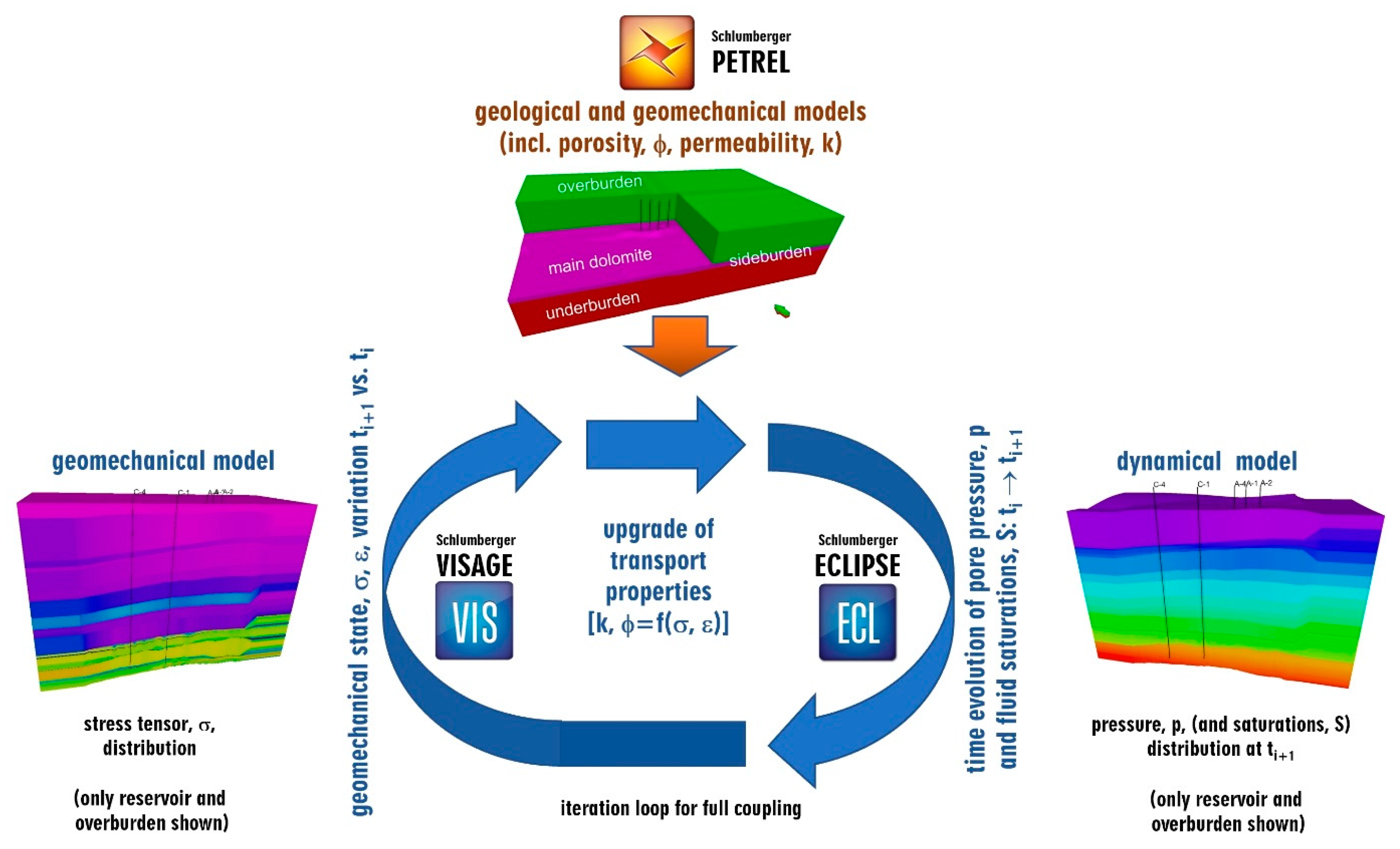
4. Geomechanic Model

During hydrocarbon production, the reservoir pressure declines, and the effective stresses increase. Conversely, during CO2 injection, to utilize the reservoir pressure as a tertiary oil recovery method (EOR) or for CO2 geological storage, there is an increase in pore pressure, which causes a decrease in the effective stresses. This effective stress principle was first proposed by Therzagi (1945) [25], which was later applied to rocks to understand their ultimate strength and ductility [26].
The change in stress within the reservoir and surrounding rocks can be expressed with an equation for isotropic rocks as follows [27]:
σ h = ν 1 ν   ( σ v α P ) + [ E 1 ν 2   ] ε h + [ E ν 1 ν 2   ] ε H
where:
σ h and σ v are the minimum horizontal and vertical stresses, respectively;
α is the Biot’s coefficient;
P is the pore pressure;
ν is the Poisson’s ratio;
E is the Young’s modulus;
σ h and ε H are the strains in the direction of the minimum and maximum horizontal stresses, respectively.
In geomechanic modelling, a set of 3D models of geomechanical parameters were developed, and then, the boundary conditions were determined to calculate the stress field and predict the geomechanical behaviour of the rock during the period of hydrocarbon production and CO2 injection into the reservoir rock.

4.1. Modelling of Geomechanical Properties

To model the distribution of geomechanical properties in 3D space, the Young’s modulus, Poisson’s ratio, unconfined compressive strength (UCS), and tensile strength were modelled in 1D for 10 boreholes before they were modelled in the geological model 3D space.

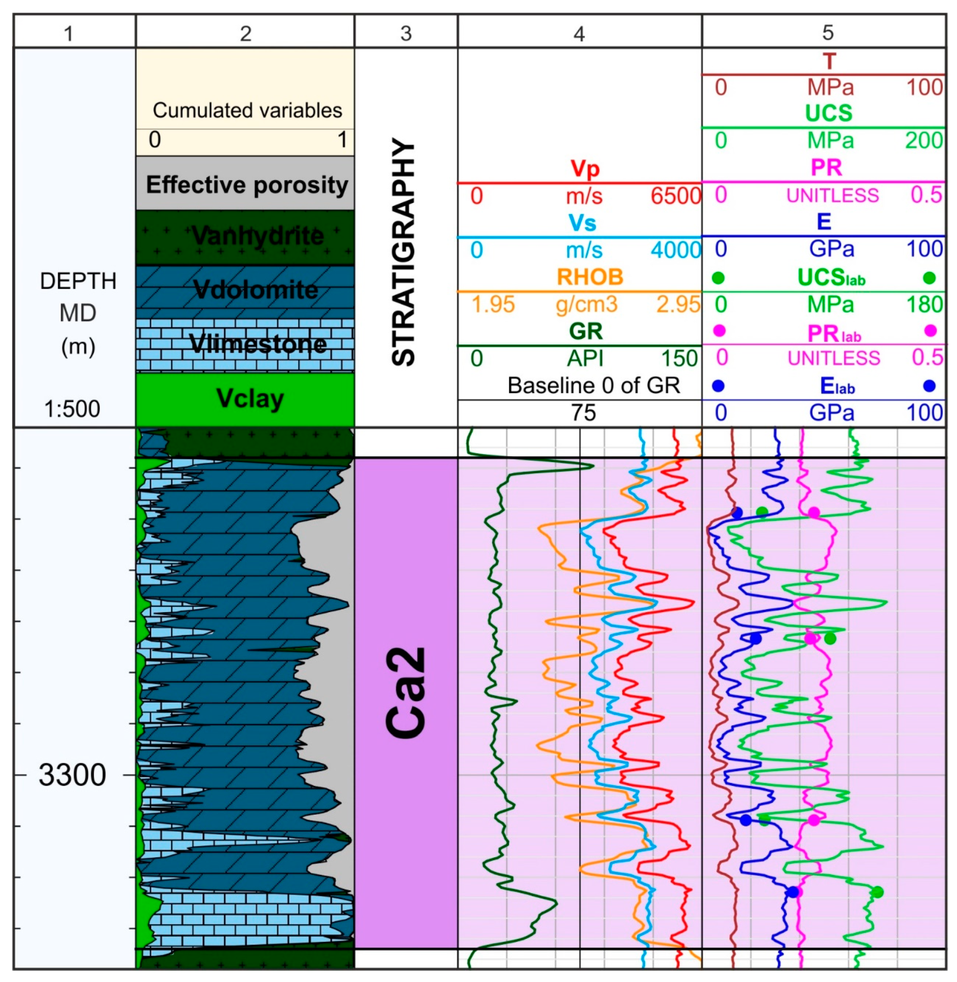
4.1.1. 1D Modelling of Elastic and Strength Properties

Herein, the models of the static elastic properties of the rocks in 1D, including Young’s modulus and Poisson’s ratio, were conducted using the well logs from 10 boreholes, the results of laboratory measurements of the static Young’s modulus parameter, and the Poisson’s ratio obtained from the core material from these boreholes. Based on the well log data, the dynamic Young’s modulus and Poisson’s ratio were calculated, wherein the relationships between the borehole velocity of the compressional vp, shear wave vs, and density ρ were used as follows [28,29,30]:
v dyn = v p 2 v s 2 2 ( v p 2 v s 2 ) ,  
E dyn = ρ   v s 2 [ ( 3 v p 2 4 v s 2 ) ( v p 2 v s 2 ) ] ,
where v dyn denotes the dynamic Poisson’s ratio, E dyn represents the dynamic Young’s modulus, v p is the velocity of the compressional wave, v s is the velocity of the shear wave, and ρ is the rock density.
The static equivalents of the elastic properties were determined by comparing the calculated dynamic properties with the results of laboratory measurements of the static elastic properties. The correlation coefficients were 0.640 and −0.588 for the Young’s modulus and Poisson’s ratio, respectively.
To estimate the static uniaxial compressive strength in the profiles of the analysed boreholes, the compressional wave velocity was compared with the results of uniaxial compressive strength laboratory measurements, which produced a linear relationship with a satisfactory correlation coefficient of 0.682.
Further, to estimate the static tensile strength, T, which was not measured on the core material, we used a simple and well-known relationship proposed by Hoek (1966) [31]:
T = UCS 10 .
As shown in Figure 6, the input data and developed 1D models of static elastic parameters, including the Poisson’s ratio, Young’s modulus, and UCS (marked with continuous line), were calibrated with the results of their measured static equivalents (marked with dots).

4.1.2. 3D Modelling of Elastic and Strength Properties

The profiles of the static geomechanical parameters from the study area were scaled up to obtain their average values along the boreholes with a defined vertical resolution of the structural model. Then, they were subjected to a geostatistical analysis, which included determining the degree of spatial correlation among the borehole data for each geomechanical parameter.
While calculating the spatial distribution of the geomechanical parameters, the truncated Gaussian simulation algorithm (TGS) with the Co-kriging option was employed, thereby allowing us to use the 3D seismic data as secondary data. The advantage of this approach is that it compensates for missing data and, therefore, unknown relationships, especially in the horizontal direction. As a result, we obtained 3D models of the geomechanical parameters, including the Young’s modulus, Poisson’s ratio, and UCS, in the main dolomite reservoir interval, as shown in Figure 7A–C, respectively. Moreover, in Figure 7D–F, the average values of the static Young’s modulus, Poisson’s ratio, and UCS in the reservoir zone, respectively, are shown.
The spatial distributions of these geomechanical properties exhibited typical relationships, in which there was a negative correlation between the elastic parameters and a positive correlation between the Young’s modulus and UCS. These relationships were also observed in the distribution of the values of these parameters illustrated as histograms. The 3D distribution of the tensile strength was obtained in a similar manner as the 1D models, wherein Hoek’s relationship with UCS was utilized. Other geomechanical parameters, such as friction angle, angle of dilatation, and the Biot’s coefficient, were assigned based on the typical values for appropriate lithologies listed in the literature [32,33,34,35,36]. The properties used as an input in the geomechanic modelling, both as a result of the modelling procedure and assumed based on the literature, are listed in Table 1.

4.2. Boundary Conditions

The boundary conditions applied to the model in order to define the initial stress for the geomechanical simulation were determined as the global tectonic stresses (minimum horizontal stress, σ h , and maximum horizontal stress, σ H ) based on a recent investigation of a tectonic stress field in Poland conducted by Jarosiński (2006) [37]. The characteristics of the assumed stress field are listed in Table 2. Note that vertical stress, σ v , is caused by gravity, and was thus determined using the overburden density (3D distribution of rock density).
The developed 3D models of the geomechanical and petrophysical parameters were used as inputs to the geomechanical simulation. These were run for seven time steps (2003, 2020, 2050, 2052, 2053, 2056, and 2100) over the course of the hydrocarbon field exploitation and CO2 injection, which were defined by the distribution of the reservoir fluid pressure developed in the reservoir fluid flow modelling. The calculated stress field reflecting the geomechanical states of the analysed rocks at specific time steps were then used to evaluate the tightness of the caprock, which could potentially leak the injected and stored CO2.

5. Dynamic Model

A dynamic model of the analysed structure was constructed using the developed geological model and was supplemented with the following additional components:
An initial distribution of reservoir fluids (oil and water) under hydrostatic conditions;
Reservoir fluid transport properties (relative permeabilities);
Reservoir fluid (oil) thermodynamic model.

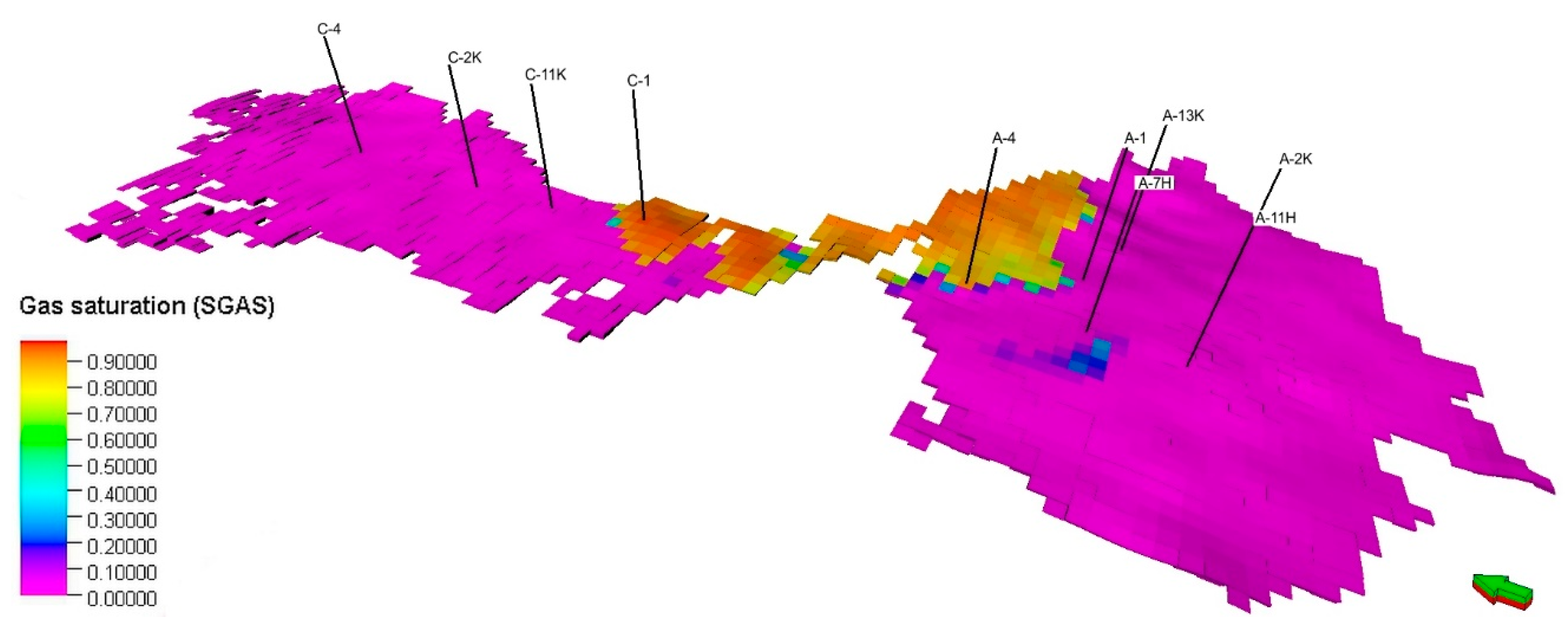
5.1. Reservoir Fluid Distributions

The presence of three reservoir fluids (water, gas, and oil) was assumed in the simulation model of the analysed reservoir. The water–oil contact was established at a depth of 3280 m b.s.l., while the gas–oil contact was established at a depth of 3178 m b.s.l. The J-Leverett function was used to generate the initial water saturation distributions that matched those obtained from the geophysical measurements. This approach enabled us to obtain the initial dynamic equilibrium by simultaneously reconstructing the water saturation values in the wells. The J-Leverett function of water saturation, Sw, considers the dependence of capillary pressure, P cow , on the parameters of the reservoir rock and has the form:
J ( S w ) = k ϕ     P cow ( S w ) σ ow cos   ( θ ow ) ,  
where k and ϕ denote the permeability and porosity of the reservoir rock, respectively, and σ ow and θ ow are the interfacial tension at the oil–water interface and their contact angle, respectively. The correct fit of the water saturation distributions in the wells was obtained using the four-parameter J curve model as follows:
J = ( A S r n + B ) ( 1 S r p ) ,   S r = S w S wc 1 S wc ,
where S wc is the connate water saturation, in which the correlation parameters were found to be: A = 0.0094, B = 0.0657, n   = 2, p = 10, and S wc = 0.0035, while σ ow = 64.65 dyne/cm and θ ow = 0 ° .
The water saturation distributions were adjusted for every well. As a result of this analysis, it was found that the model correctly reproduced the water saturation variation with depth in most wells. As a result, the average water saturation in the model generated corresponds with high accuracy to the average water saturation generated using the interpolation method in the geological model.

5.2. Transport Properties

In general, transport properties in porous media include various flow mechanisms ranging from continuous flow of viscous type (Darcy flow) through slippage effects to Knudsen and molecular diffusion. Similarly, thermodynamics associated with transport phenomena may obey classical laws of locally equilibration state for large porosity systems and follow non-equilibrium type for small porosity system where molecule collisions with the walls of the system dominates over inter-particle ones. In contrast to low permeability, low porosity rocks [38,39] (tight and shale formations), conventional rocks such as dolomites included in the analysed case reveal standard viscous flow characterized by permeability tensors and equilibrium thermodynamic variables like pressure drop and shear stress. The other type of rocks in the analysed model refers to caprock anhydrite. Although it is an extremally low permeability rock, its main feature used in this study concerns the dependence of transport properties upon geomechanical state that was established in terms of effective permeability [13]. Consequently, in order to model effects of gas transport across the anhydrite caprock, a conventional approach was applied adopting stress-dependent permeability of a single porosity micro-fractured system.
An important part of the transport described by permeabilities is played by relative permeabilities of various reservoir fluids. Owing to the lack of direct measurements of the relative permeability curves, kr, and reduced fluid saturation, Sr, for the analysed reservoir, a power model was adopted according to the relationship: kr = (Sr)n, wherein reduced saturation was determined as follows:
S r = S S min S max S min ,
where Smin and Smax refer to the minimum and maximum available saturations, respectively. The model used the following parameter values: for water (kr = krw, S = Sw): irreducible water saturation Smin = Swcr = 0.0528, maximum water saturation, Smax = 1; for oil in the oil–water system (with no gas kr = krow, S = So): Smin = Sorw = 0.4917, Smax = Somax = 1 − Swco = 0.9964; for oil in the oil–gas system (at connate water saturation, kr = krog, S = So) Smin = Sorw + Swco, Smax = Somax; and for gas in the oil–gas/water–gas system (kr = krg, S = Sg) Smin = Sgcr = 0.1, Smax = Sgmax = 1 − Swco = 0.9964. Both the exponent of the relationship and the other parameters were adjusted during the model calibration procedure.

5.3. Reservoir Fluid Model

As the simulation model of the analysed reservoir (structure) is compositional, a thermodynamic model of the reservoir fluid (oil and gas) was constructed and calibrated based on the Soave–Redlich–Kwong (SRK) equation of state (EoS) using a standard software tool (PVTSim software, [40]). SRK equation of state is a conventional equation that relates temperature, pressure and volume of fluid and uses two parameters taking into account interaction of fluid molecules and their volumes. Those parameters are expressed in terms of several physical quantities, such as critical pressure, temperature, and volume. Other quantities include eccentricity factors [41], molar masses and boiling point temperatures. All these quantities are well defined for single component fluids such as light hydrocarbons (up to C6) and non-hydrocarbon components (N2, CO2, H2S). For heavier hydrocarbons they are determined by empirical correlations with densities and molar masses [42]. In order to effectively perform compositional reservoir simulations, the number of fluid components is typically reduced by grouping or lumping the heavier ones. Effective parameters of such pseudo-components are calculated as averages of the real components with weights proportional to their concentrations and molar masses. In addition, the equation of state for multicomponent mixtures includes interaction effects of different polar molecules by so called mixing rules expressed via binary coefficients [43]. The viscosities of gas and liquid phases of the analysed fluid were determined using Lohrenz–Bray–Clark correlation [44] of viscosity and density and the results of the SRK equation of state for the densities. The SRK equation of state with parameters described above is typically sufficient to predict fluid properties. However, its results can be improved by the method of EoS regression [45] to experimental data.
In the analysed case the original fluid model [46] included 25 components determined by chromatographic analysis (gas phase components) and true boiling point analysis (liquid phase components) that were subsequently grouped into eight effective components, as summarized in Table 3.
The model was calibrated using the regression method to the following experimental data: the pressure at the saturation point, constant mass expansion tests (relative volumes of gas and liquid phases, effective compressibilities), differential depletion tests (oil and gas formation volume factors, gas-in-oil solubility, oil density, gas z-factor, oil and gas viscosities, gas gravity), separator tests (gas–oil ratio, gas gravity, oil formation volume factor), and viscosity tests (oil viscosity).
The following regression parameters of the SRK EoS were used: critical temperatures and pressures, eccentricity and ΩA factors of 2 grouped components (C7–C11, C12+)—the complete set of the EoS parameters and their values are given in Table 4 and Table 5. Additional regression parameters were those of Lohrenz–Bray–Clark correlation coefficients—given in Table 6.

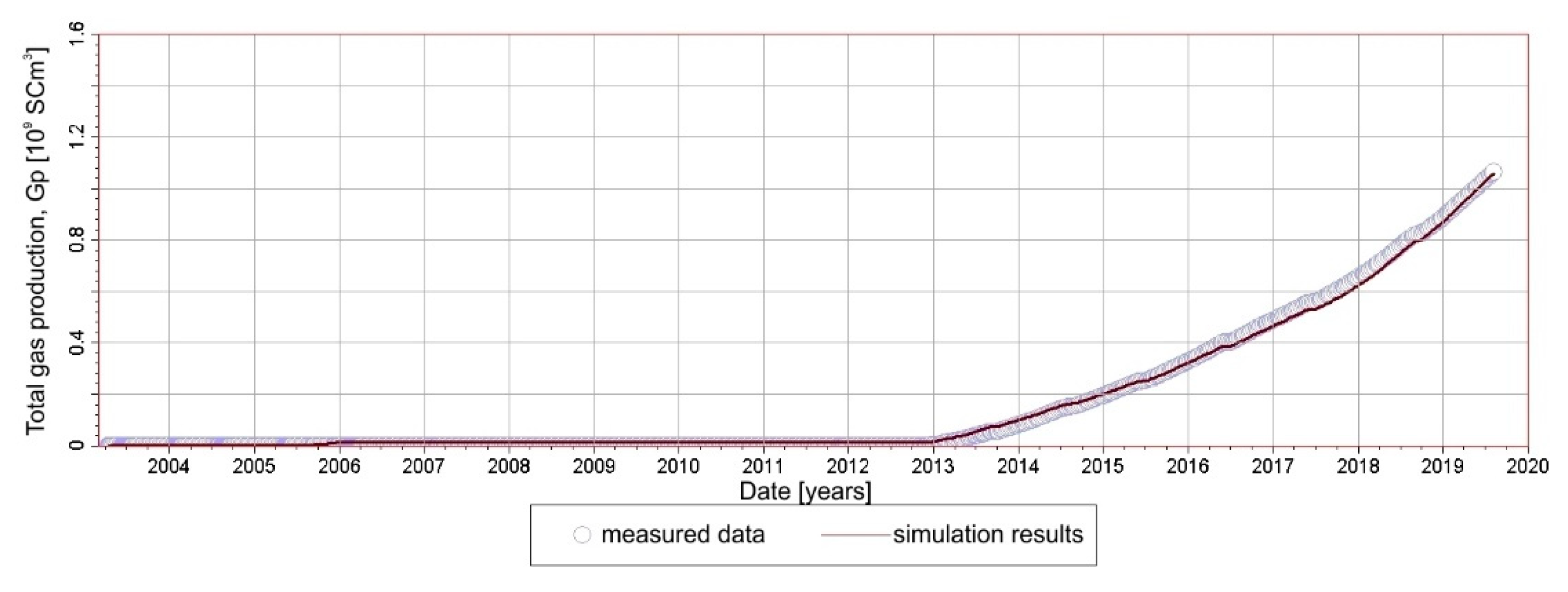
6. Model Calibration

The model of the analysed reservoir was calibrated against the production data covering 16 years of operation with 11 producing wells. The data included daily oil, gas, and water production rates from individual wells, bottom-hole pressures, and well test results.

6.1. Calibration Results

Model calibration involved modifying the following model parameters: global and local petrophysical parameters (absolute and relative permeabilities and permeability anisotropies), well productivity indices, and skin-effect coefficients. As a result, a significant increase in the gas–oil-ratio (GOR) during operation was reproduced for wells C-1, A-1, and A-4, which were located directly or in the vicinity of the primary gas cap (Figure 8), and for the wells located relatively far away from the primary gas cap but influenced by the formation of a secondary gas cap.
The necessity to accurately reproduce the measured bottom-hole pressures required a linear characteristic of the relative gas permeability at the top zone of the structure, which suggests the existence of micro-fractures in the reservoir. The critical oil saturation was found to be consistent with the results obtained from the laboratory experiments regarding oil displacement with water. Further, the permeability vertical-to-horizontal anisotropy increased, which resulted in the correct depression in the production wells and reduced the migration of the released gas to the top of the structure.
Acid treatments of wells C-1, C-2k, and A-4 were modelled by modifying the absolute permeability and effective pore volume in their near-wellbore zones. To reproduce the relatively high pressure difference measured between the C-1, C-2k, and C-11k wells, deteriorated petrophysical properties were introduced among these wells. A local reduction in the absolute permeability anisotropy near the A-11H and A-13k wells caused the simulated results of the GOR to become closer to the observed values. In general, the productivity indices and skin-effect coefficients of the wells were accordingly adjusted to the depressions observed during the well tests.
Figure 9 and Figure 10 present the total oil and gas production from the field as a result of the calibrated simulation model versus the measured values, revealing that the model matched the production data with high accuracy. At the well level, Figure 11 shows an example of the adjustment quality of the bottom-hole pressures measured at a production well. Meanwhile, as shown in Figure 12, good GOR fitting in an individual well was achieved. Further, Figure 13 shows an example of the adjustments to the bottom-hole pressure evolution reported during the well production test. Thus, the simulation results are in good agreement with the measured values for all the available historical production data.

6.2. Model Characterisation after Calibration

After the calibration process, the simulation model of the analysed reservoir was characterised by the following parameters: total area: 15 km × 10 km, the nature of the model: single porosity and permeability, lateral dimensions: 376 blocks × 242 blocks, lateral sizes of the blocks: 100 m × 100 m, layer structure: 15 layers, number of active blocks: 20,325, initial contact depths: oil–water: 3282 m b.s.l., gas–oil: 3178 m b.s.l., initial pressure: 430.2 bar (@ 3282 m b.s.l.), reservoir temperature (constant): 126.8 °C, total model pore volume: 70.2 million m3, average values of basic parameters: porosity: 9.6%, horizontal permeability: 34.91 mD, vertical permeability: 1.4 mD, and total thickness of a simulation layer: 2.77 m.

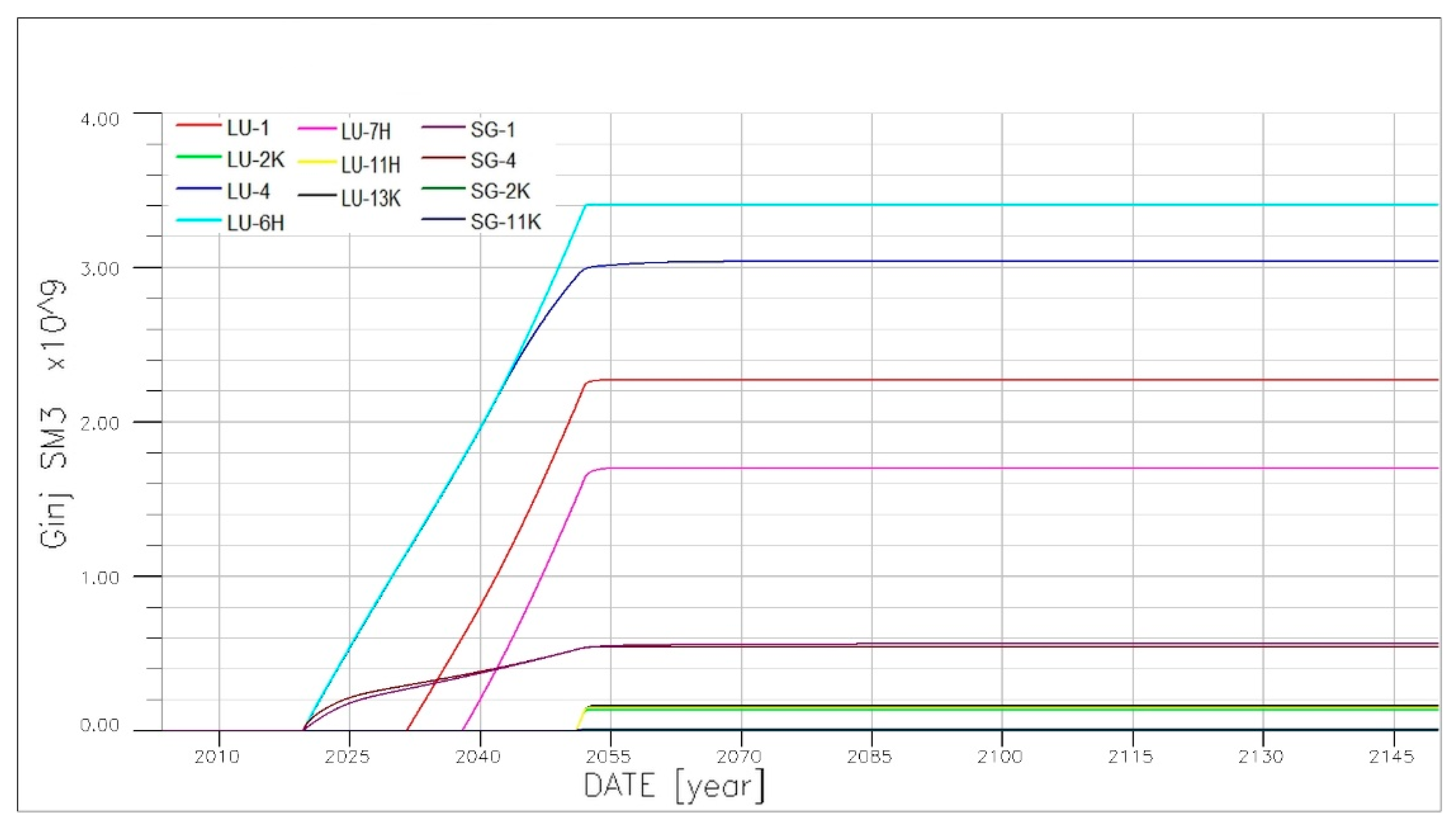
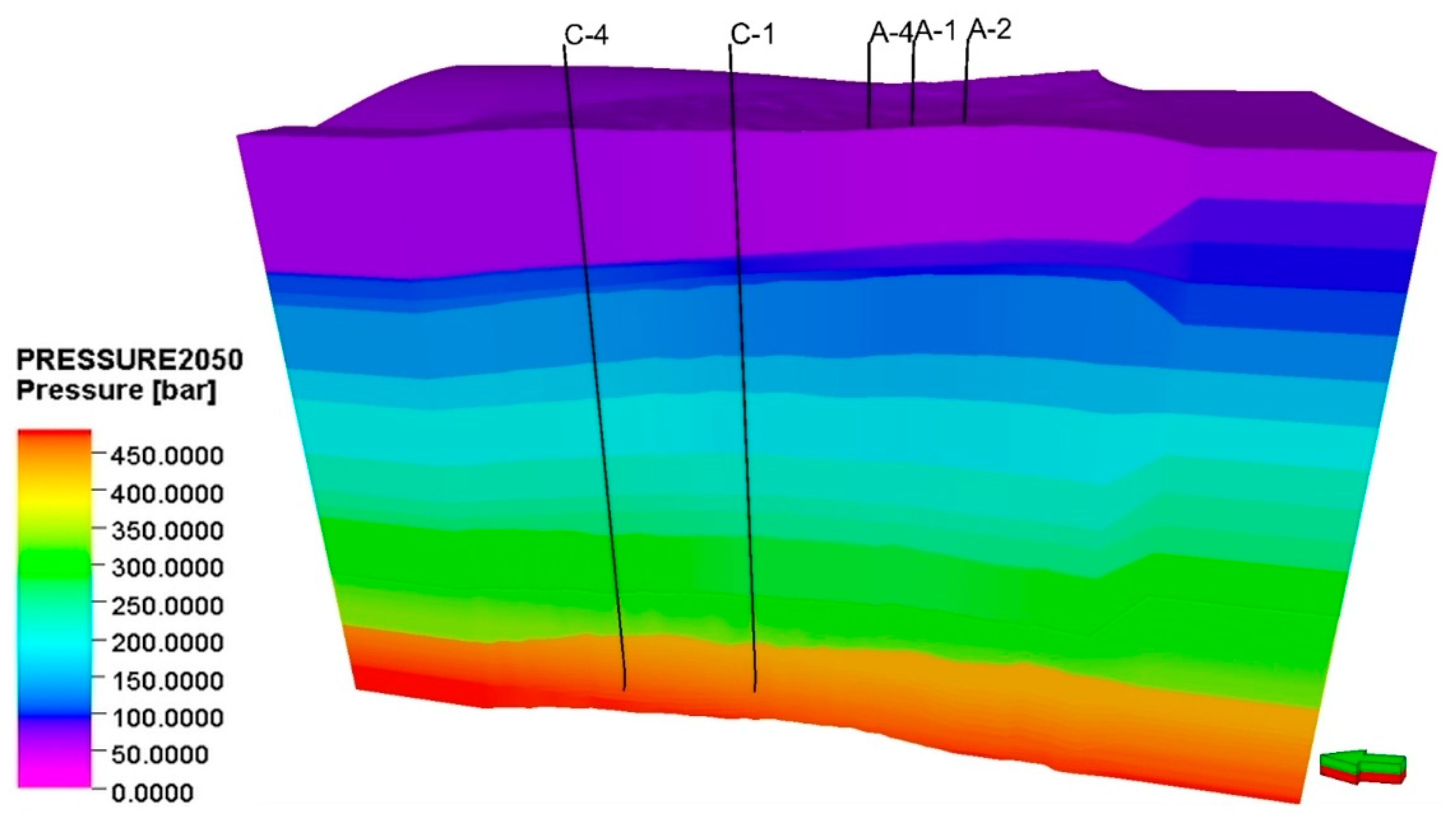
7. Pressure Evolution

The dynamic flow model of the analysed reservoir was used to simulate the reservoir behaviour during enhanced oil recovery with CO2 injection followed by exclusive CO2 injection. Production rates of the oil producing wells were assumed at the nominal levels provided by the reservoir operator. In addition, they were constrained by the minimum well-head pressure, maximum water cut, maximum gas oil ratio, minimum economic flow rate, and maximum allowable drawdown. Initially, CO2 injection was performed using four wells (A-4, A-6H, C-1, and C-4), before injection expanded to other wells, which were converted from producing wells after they ceased production. The injection rates of individual wells were controlled by the total injection rate and well contributions proportional to their injectivities. The injecting wells were constrained by the maximum bottom-hole pressures not exceeding the formation fracturing pressure. The injection phase lasted approximately 36 years. As a result of the simulation of this EOR/CO2 sequestration project (called the basic scenario), all the significant quantities characterising the project were obtained. Figure 14 shows the total oil production and average reservoir pressure evolution during the project.
The contributions of individual wells to the reservoir oil production are shown in Figure 15 in terms of their total oil production.
The quantitative characteristics of the CO2 injection process were expressed as the total CO2 injection of the project and as the total CO2 injection of individual wells, as shown in Figure 16 and Figure 17, respectively.
Figure 18 shows the effects of EOR with CO2 injection by comparing the total oil production of this project with total oil production using the primary oil production method. The incremental oil production exceeds 6.3 × 10⁶ Sm3, which is equivalent to approximately 130% of the primary production (4.8 × 10⁶ Sm3).
The simulation results include pressure distributions across the analysed structure extended model at various stages of the EOR/CO2 sequestration project, as shown in Figure 19.
To present a more detailed variation in the pressure distribution, pressure maps for the top layer of the reservoir are shown in Figure 20 for various stages of the project.

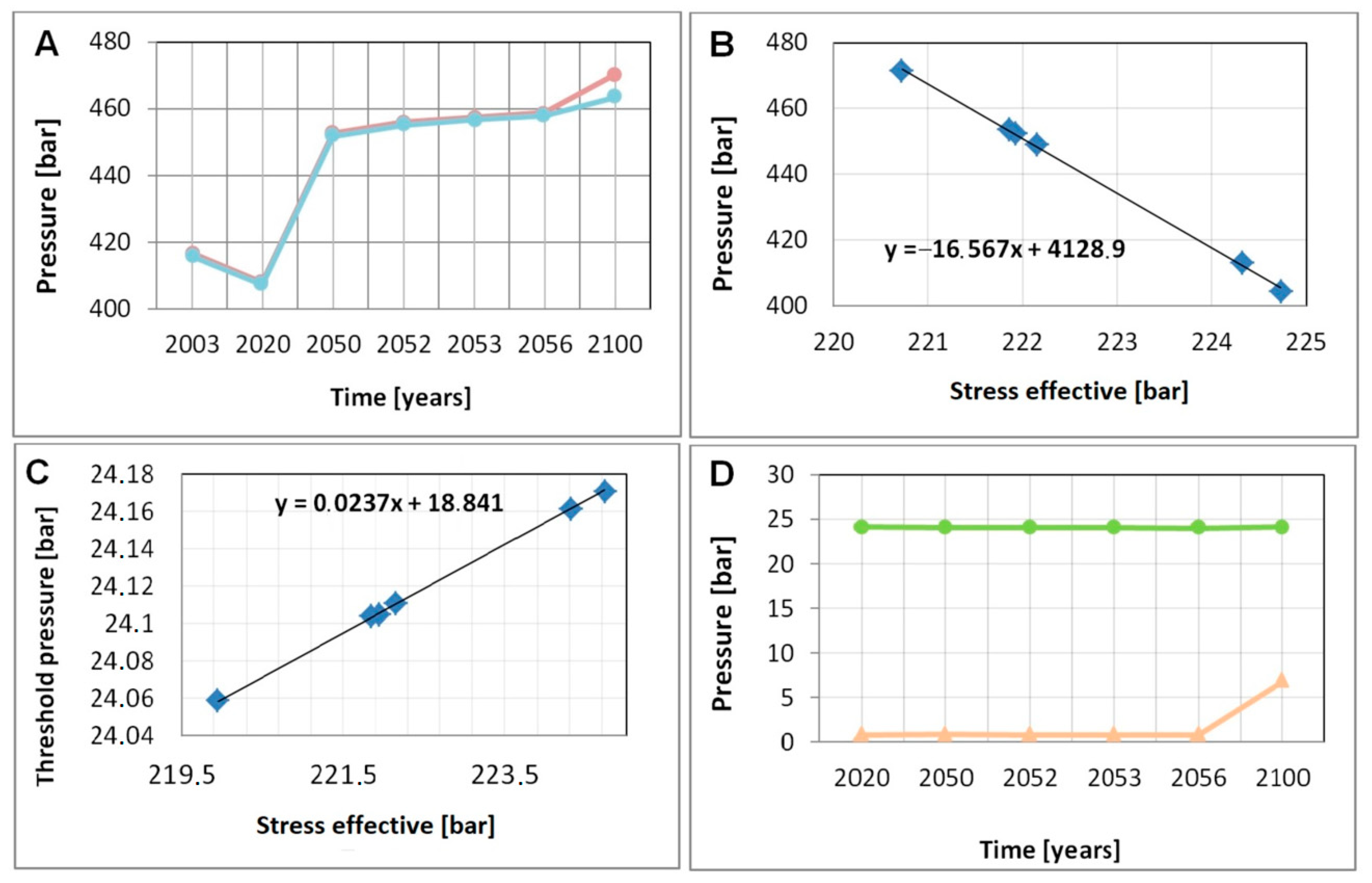
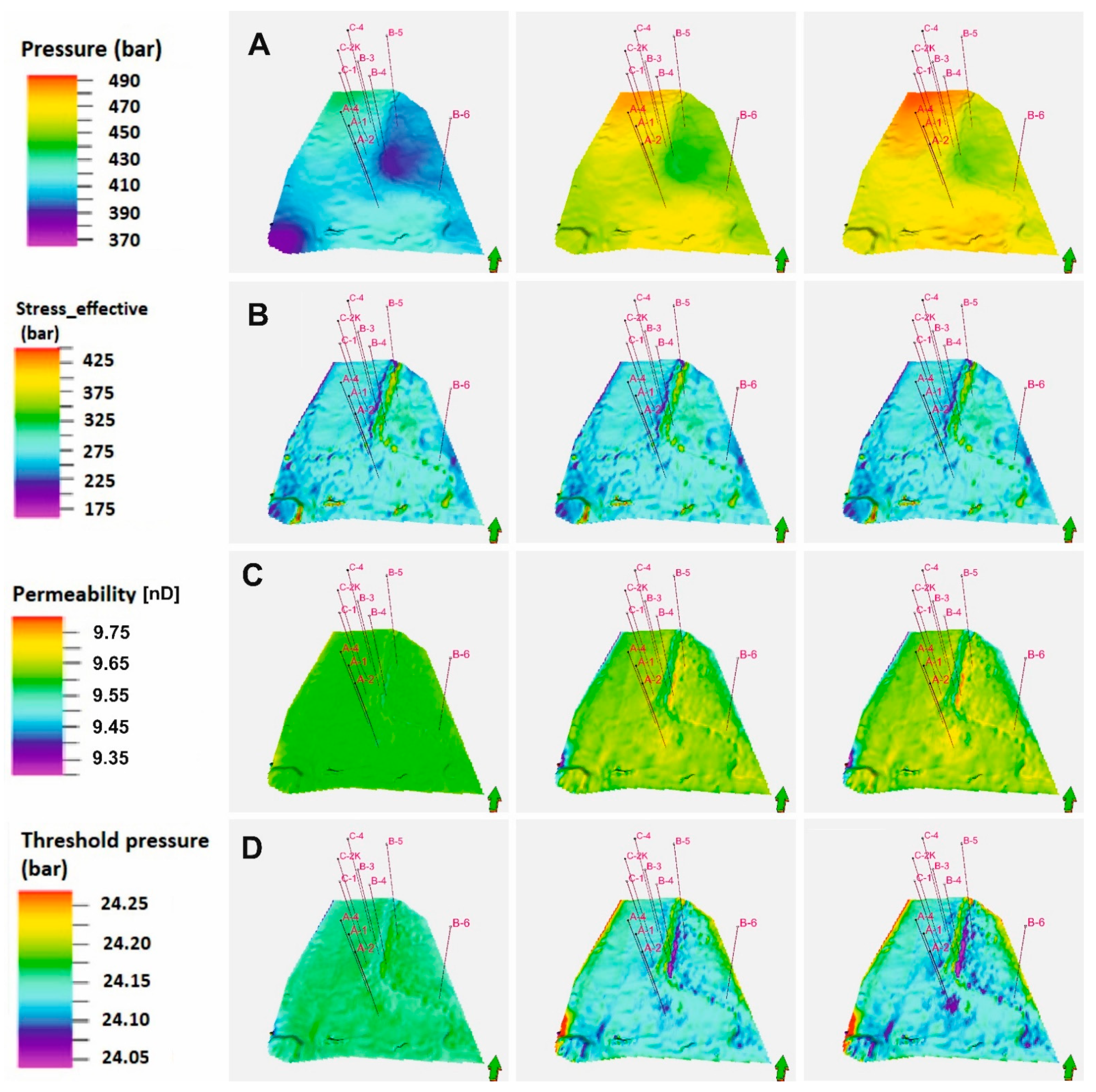
8. Caprock Sealing Analysis

The migration of stored CO2 into the overlying strata is inhibited by the sealing properties of very low permeability and high capillary forces, which prevent gas penetration into the water-saturated caprock. The parameter governing this sealing ability is the threshold pressure. If the value of the threshold caprock pressure exceeds that of the gas, the caprock pores begin to be penetrated, ultimately leading to the development of interconnected pathways for gas to escape upward [47]. This threshold pressure can be measured using the method first proposed by Thomas et al. (1968) [48], which was later modified using empirical models adopted for a specific lithology. In general, among the different lithologies, anhydrites, carbonates, and shales have high threshold pressure and low permeability, making them potentially good sealing rocks for gas storage.
In this study, to calculate the threshold pressure in the basal anhydrite (A2), a direct sealing layer neighbouring the reservoir rock, we used the empirical relationship as follows:
P th = a   k b ,
where P th is the threshold pressure, k is the permeability, a is the multiplication coefficient, and b is the exponent. The coefficients a and b were developed by Ibrahim et al. (1970) [49], who studied seven samples of anhydrites. The permeability in the history of reservoir exploitation and forecasting of CO2 injection into the main dolomite reservoir rock was estimated based on the stress dependency on permeability, wherein the stress variation was obtained using geomechanical simulations.
Numerous scientific investigations have revealed that both porosity and permeability are affected by dominant loading conditions and the history of stresses within the sedimentary basin. This relationship is widely known and well documented [13,50,51,52]. Based on the laboratory permeability measurements performed by Morrow et al. (1984) for fault gouges [53], Shi and Wang (1988) suggested that the power law describes the nonlinear decline in permeability with increasing effective stress in the low-permeability rocks well in the following form [50]:
k = k 0 ( σ σ 0 ) p ,
where k denotes the permeability under effective stress σ , k 0 is the initial permeability at the initial effective stress σ 0 , and p is the material constant. Regarding effective stress, we used the magnitude of the minimum horizontal stress as it is mostly responsible for the decline in permeability in the mechanism of closing microcracks potentially present in the anhydrite rocks.
As the data regarding the petrophysical characteristics of the Zechstein anhydrites in Poland were not available, we used a typical value of permeability for anhydrites [54] and the material constant p determined by Zivara et al. (2019) [13]. The results of geomechanical simulations performed for the selected time steps provided the distribution of effective stresses evolving throughout the CO2 injection operation. The calculated permeability was then used to estimate the threshold pressure at selected time steps, ending approximately 80 years after the initial CO2 injection.
Table 7 lists the assumed values of initial permeability, material constant, and the other coefficients employed for the threshold pressure calculation in the basal anhydrite (A2).
As shown in Figure 21, the evolution of pressure in the selected location at the top of the reservoir Ca2 (red line) and in the basal anhydrite A2 (blue line) exhibit a negative correlation between the magnitude of the minimum horizontal stress and reservoir pressure, a positive relationship between the magnitude of the minimum horizontal stress and the threshold pressure and the evolution of the threshold pressure (green line), and a pressure step between the top of the reservoir and basal anhydrite (orange line).
The spatial distributions of the pressure (A), magnitude of the minimum horizontal stress (B), estimated permeability (C), and calculated threshold pressure (D) for the time steps representing the end of hydrocarbon production (2020—left column), during the process of CO2 injection (2056—middle column), and at the end of CO2 injection (2100—right column) in the sealing anhydrite (A2) are shown in Figure 22.
These distributions show that the increase in pore pressure in the sealing rock along with the injection of CO2 in the reservoir zone caused a very slight increase in effective stress and, consequently, a small increase in the permeability, from 9.55 nD to 9.80 nD. This change results in a small decrease in the threshold pressure, from 24.16 bar to 24.05 bar. These changes are small and local, and the threshold pressure remains at a safe level of approximately 24 bars. The most sensitive area is localised within the slope of the platform, near injection wells B-4 and B-5. The increase in permeability (yellow-red colour) and decline in threshold pressure (purple colour) were significant in this area. Another sensitive zone is located in the deep-water zone near injection wells A1, A2, and A-4.
The difference between the pressure in the top layer of the reservoir (Ca2) and the sealing layer of the basal anhydrite (A2) shown in Figure 23 helped to determine where additional CO2 can be injected without exceeding the threshold pressure in the anhydrite, thereby lowering the risk of CO2 leakage.

9. Gas Leakage Analysis

In addition to caprock sealing conditions, the quantitative studies of gas leakage to the caprock were performed using the structure simulation model described above. As the caprock maintains its sealing properties up to the determined threshold pressure, the leakage occurs only when the pressure step across the caprock-reservoir boundary exceeds the threshold pressure. In this section, the quantitative results of the leakage to the caprock were determined for several scenarios, characterised by varying amounts of injected/sequestrated CO2 as listed in Table 8. The varying amounts of total injection/sequestration were realised by the modifications of the well group injection rate. All the other constraints were kept unchanged.
The progress of the CO2 injection process was presented in Figure 24 and Figure 25 in terms of time evolution for total CO2 injection and average reservoir pressure, respectively.
The detailed pressure distribution at the reservoir top revealed a pressure step across the reservoir–caprock boundary exceeding the threshold pressure at several locations. As a consequence, CO2 leaked from the reservoir to the overlying anhydrite layers. The effects of this leakage process are shown in Figure 26 for each of the four scenarios considered. The final (140 years after the injection finish) amounts of the total leakage and their value as a fraction of injected CO2 are listed in Table 9.
Although the CO2 leakage rate gradually decreased with time, it continued up to the extended end of the simulation period (140 years of relaxation phase after the injection finish). Note that the leaked CO2 accumulated in the bottom layer of the anhydrite horizon, wherein a relatively small amount (2.5%) of CO2 reached the anhydrite top, as shown in Figure 27.
The process of CO2 leakage from the reservoir to the caprock was very heterogeneous because of the following:
inhomogeneous reservoir rock properties,
varying depths of the reservoir-caprock boundary,
inhomogeneity of the CO2 injection process.
The detailed distributions of CO2 saturation at the end of the simulation period found in the top layer of the reservoir and the three layers composing the anhydrite horizon are shown in Figure 28 for the selected scenarios.

10. Summary and Conclusions

The studies described herein address the practical problem of geological structure tightness for the purpose of CO2 sequestration applied to a geological structure to be assessed as the potential site of a future sequestration project. The studies took the advantage of advanced methods, realistic assumptions, and quantitative results of previous, general studies to practically evaluate the operation of the real geological structure of a domestic oil reservoir including the initial phase of enhanced oil recovery by CO2 injection and final phase of CO2 sequestration.
In particular, we performed an analysis of the tightness of the basal anhydrite (A2), which is the sealing layer for the hydrocarbon accumulation in the main dolomite formation (Ca2). To this end, we used numerical methods that combined geomechanical and reservoir fluid flow modelling. Based on a large set of data, geological, structural, and parametric models were developed. To predict the reservoir and surrounding rock behaviour caused by CO2 injection, dynamic flow and geomechanical models were constructed based on the geological model supplemented by all the other required components. These models were satisfactorily matched with the historical reservoir operation data. Then, the models were used to forecast the reservoir behaviour (evolution of detailed pressure and fluid saturation distributions) under the assumptions of an EOR project with CO2 injection followed by a CO2 sequestration phase. The dynamic simulations were combined with the geomechanical simulations using a two-way coupling procedure and utilising correlations between the geomechanical state (stress and strain distribution) and transport properties of the reservoir rock and caprock, including the threshold pressure at the reservoir–caprock boundary.
The results of the procedure determined the sequestration capacity of the structure. In addition, the effects of CO2 leakage from the reservoir to the caprock were simulated in cases where the reservoir pressure at the structure top (reservoir–caprock boundary) exceeded the limits of the threshold pressure. The long-term simulations resulted in an assessment of the total amount of CO2 leakage and its distribution within the caprock horizon as a function of time for various total CO2 injection volumes above the sequestration capacity.
Based on the simulation results, the following conclusions can be drawn:
(1)
General conclusions:
The method applied in the studies proves the necessity to employ an extended model of the analysed structure, wherein the geomechanical and dynamical simulations allow precise estimations of the threshold pressure and provide information regarding critical locations at the reservoir–caprock boundary where leakage could occur.
The precise determination of the threshold pressure (with inhomogeneous distribution across the reservoir–caprock boundary) and its evolution with time are crucial factors for estimating the sequestration capacity of the structure.
The following two correlations are key factors when the sealing properties of the reservoir caprock boundary are evaluated:
  • The correlation between the geomechanical state (stress field) and transport properties (permeabilities) of the caprock;
  • The correlation between the caprock permeability and threshold pressure at the reservoir-caprock boundary.
(2)
Conclusions specific to the analysed geological structure:
The determined threshold pressure revealed the potential CO2 sequestration capacity of the structure, showing that it could safely store approximately 12 × 109 Sm3 of gas.
The relatively low (up to 3.6%) excess over the determined sequestration capacity resulted in a very small total CO2 leakage (0.13‰ of the sequestrated volume) up to approximately 100 years of relaxation phase after CO2 injection is complete.
Most of the leaked CO2 accumulates in the bottom part of the caprock.
The leakage process does not cease even at the end of the simulated (100 years) relaxation phase.

Author Contributions

Conceptualization, M.S.-V., W.S. and A.G.; methodology, M.S.-V., W.S. and A.G.; software, M.S.-V., K.S. and A.G.; validation, M.S.-V. and W.S.; formal analysis, M.S.-V., W.S. and A.G.; investigation, M.S.-V. and A.G.; resources, M.S.-V. and A.G.; data curation, M.S.-V., K.S. and A.G.; writing—original draft preparation, M.S.-V., W.S. and K.S.; writing—review and editing, M.S.-V. and W.S.; visualization, M.S.-V., A.G. and K.S.; supervision, K.S. and W.S.; project administration, M.S.-V. All authors have read and agreed to the published version of the manuscript.

Funding

This research was carried out as part of the ‘Analysis of geological structure tightness for the purposes of CO2 sequestration’ project, which is funded by the Polish Ministry of Science and Higher Education, Grant No. DK-4100-39/20. The authors would like to express their gratitude to the Polish Ministry of Science and Higher Education for funding this research.

Institutional Review Board Statement

Not applicable.

Informed Consent Statement

Not applicable.

Data Availability Statement

The data that support the findings of this study are available on reasonable request from the corresponding author.

Conflicts of Interest

The authors declare no conflict of interest.

Abbreviations

SCm3Standard cubic meter
ƐHThe strains in the direction of the maximum horizontal stress
ƐhThe strains in the direction of the minimum horizontal stress
pThe material constant
A1DThe lower Anhydrite of Werra cyclothem
A1GThe upper Anhydrite of Werra cyclothem
A2The basal Anhydrite of Stassfurt cyclothem
A2GScreening Anhydrite of Stassfurt cyclothem
A3The main Anhydrite of Leine cyclothem
A4DThe lower Anhydrite of Aller cyclothem
A4GThe upper Anhydrite of Aller cyclothem
Ca1Zechstein limestone of Werra cyclothem
Ca2The main Dolomite of Stassfurt cyclothem
EYoung’s modulus
EOREnhanced oil recovery method
FGITTotal CO2 injection
FGPT Total gas production
FOPTTotal oil production
FPRAverage reservoir pressure
GinTotal CO2 injection of individual wells
GORGas to oil ratio
GRNatural Gamma radiation
I3Salt clay of Leine cyclothem
kPermeability of the rock
k0The initial permeability
MMolar mass
Na1The oldest Halite of Werra cyclothem
Na2Older Halite of Stassfurt cyclothem
Na4The youngest Halite of Aller cyclothem
PPore pressure
PcowCapillary pressure
PcCritical pressure
PthThe threshold pressure
PVT Pressure, volume and temperature
PZ2Stassfurt cyclothem
PZ3Leine cyclothem
PZ4Aller cyclothem
SmaxThe maximum available saturations
SminThe minimum available saturations
SRK EoSSoave–Redlich–Kwong equation of state
SwWater saturation
SwcThe connate water saturation
TTensile strength
TbBoiling point
TcCritical temperature
TGSTruncated Gaussian Simulation algorithm
UCSUniaxial compressive strength
VcCritical volume
vpCompressional wave velocity
vsShear wave velocity
ZcCritical gas compressibility factor
αThe Biot’s coefficient
θowOil-water contact angle
νPoisson’s ratio (PR)
ρRock density (RHOB)
σeffEffective stress
σHThe maximum horizontal stress
σhThe minimum horizontal stress
σvThe vertical stress
σ0Initial effective stress
σowInterfacial tension at the oil–water interface
φPorosity of the rock
ωEccentricity factor

References

  1. Hangx, S.J.T.; Spiers, C.J. Reaction of plagioclase feldspars with CO2 under hydrothermal conditions. Chem. Geol. 2009, 265, 88–98. [Google Scholar] [CrossRef]
  2. Bang, J.-H.; Chae, S.C.; Lee, S.-W.; Kim, J.-W.; Song, K.; Kim, J.; Kim, W. Sequential carbonate mineralization of desalination brine for CO2 emission reduction. J. CO2 Util. 2019, 33, 427–433. [Google Scholar] [CrossRef]
  3. Qanbari, F.; Pooladi-Darvish, M.; Tabatabaie, S.H.; Gerami, S. CO2 disposal as hydrate in ocean sediments. J. Nat. Gas Sci. Eng. 2012, 8, 139–149. [Google Scholar] [CrossRef]
  4. Power, I.M.; Dipple, G.M.; Bradshaw, P.M.; Harrison, A.L. Prospects for CO2 mineralization and enhanced weathering of ultramafic mine tailings from the Baptiste nickel deposit in British Columbia, Canada. Int. J. Greenh. Gas Control 2020, 94, 102895. [Google Scholar] [CrossRef]
  5. Zhang, D.; Zhao, Z.-Q.; Li, X.-D.; Zhang, L.-L.; Chen, A.-C. Assessing the oxidative weathering of pyrite and its role in controlling atmospheric CO2 release in the eastern Qinghai-Tibet Plateau. Chem. Geol. 2020, 543, 119605. [Google Scholar] [CrossRef]
  6. Li, D.; Saraji, S.; Jiao, Z.; Zhang, Y. CO2 injection strategies for enhanced oil recovery and geological sequestration in a tight reservoir: An experimental study. Fuel 2021, 284, 119013. [Google Scholar] [CrossRef]
  7. Wójcicki, A. Assessment of Formations and Structures Suitable for Safe CO2 Geological Storage (in Poland) including the Monitoring Plans, Final Report. Rozpoznanie Formacji I Struktur Do Bezpiecznego Geologicznego Składowania CO2 Wraz Z Ich Programem Monitorowania, Raport Końcowy; Strona Projektu: Warsaw, Poland, 2013. Available online: http://skladowanie.pgi.gov.pl (accessed on 25 July 2020).
  8. Chadwick, A.; Arts, R.; Bernstone, C.; May, F.; Thibeau, S.; Zweigel, P. Best Practice for the Storage of CO2 in Saline Aquifers, Observations and Guidelines from the SACS and CO2STORE Projects; British Geological Survey; Halstan & Co. Ltd.: Amersham, UK, 2008. [Google Scholar]
  9. Tarkowski, R.; Stopa, J. Tightness of geological structure destined to underground carbon dioxide storage. Gospod. Surowcami Miner. Resour. Manag. 2007, 23, 129–137. [Google Scholar]
  10. Lubaś, J.; Szott, W. 15-year experience of acid gas storage in the natural gas structure of Borzęcin—Poland. Nafta-Gaz 2010, 66, 333–338. [Google Scholar]
  11. Edlmann, K.; Haszeldine, S.; McDermott, C.I. Experimental investigation into the sealing capability of naturally fractured shale caprocks to supercritical carbon dioxide flow. Environ. Earth Sci. 2013, 70, 3393–3409. [Google Scholar] [CrossRef] [Green Version]
  12. Li, Z.; Dong, M.; Li, S.; Huang, S. CO2 sequestration in depleted oil and gas reservoirs—caprock characterization and storage capacity. Energy Convers. Manag. 2006, 47, 1372–1382. [Google Scholar] [CrossRef]
  13. Zivar, D.; Foroozesha, J.; Pourafsharyb, P.; Salmanpour, S. Stress dependency of permeability, porosity and flow channels in anhydrite and carbonate rocks. J. Nat. Gas Sci. Eng. 2019, 70, 1–13. [Google Scholar] [CrossRef]
  14. Hangx, S.; Spiers, C.; Peach, C. The mechanical behavior of anhydrite and the effect of CO2 Injection. Energy Procedia 2009, 1, 3485–3492. [Google Scholar] [CrossRef] [Green Version]
  15. Jaskowiak, S.M.; Karaczun, K.; Karaczun, M.; Grobelny, A.; Jankowski, H.; Mlynarski, S.; Kuhn, D.; Pokorski, A.; Wagner, R.; Gajewska, I.; et al. Budowa geologiczna niecki szczecińskiej i bloku Gorzowa. Inst. Geol. Czech Acad. Sci. 1979, 96, 178. [Google Scholar]
  16. Czekański, E.; Kwolek, K.; Mikołajewski, Z. Hydrocarbon fields in the Zechstein Main Dolomite (Ca2) on the Gorzów Block (NW Poland). Przegląd Geol. 2010, 58, 695–703. [Google Scholar]
  17. Peryt, T.M.; Dyjaczyński, K. An isolated carbonate bank in the Zechstein Main Dolomite basin, western Poland. J. Pet. Geol. 1991, 14, 445–458. [Google Scholar] [CrossRef]
  18. Protas, A.; Wojtkowiak, Z.; Blok, G. Geologia dolnego cechsztynu. In Przewodnik LXXI Zjazdu Polskiego Towarzystwa Geolog-Icznego; Wydawnictwo Instytutu Naukowo Geologicznego: Poznań, Poland, 2000; ISBN 8388163388. [Google Scholar]
  19. Jaworowski, K.; Mikołajewski, Z. Oil- and gas-bearing sediments of the Main Dolomite (Ca2) in the Międzychód region: A depositional model and the problem of the boundary between the second and third depositional sequences in the Polish Zechstein Basin. Przegląd Geol. 2007, 55, 1017–1024. [Google Scholar]
  20. Słowakiewicz, M.; Mikołajewski, Z. Sequence stratigraphy of the Upper Permian Zechstein Main Dolomite carbonates in Western Poland: A new approach. J. Pet. Geol. 2009, 32, 215–234. [Google Scholar] [CrossRef]
  21. Słowakiewicz, M.; Mikołajewski, Z. Upper Permian Main Dolomite microbial carbonates as potential source rocks for hydrocarbons (W Poland). Mar. Pet. Geol. 2011, 28, 1572–1591. [Google Scholar] [CrossRef]
  22. Wagner, R. Stratigraphy of Deposits and Evolution of the Zechstein Basin in the Polish Lowlands. Stratygrafia Osadów I Rozwój Basenu Cechsztyńskiego Na Niżu Polskim: Prace Państwowego Instytutu Geologicznego; Państwowy Inst. Geologiczny: Warszawa, Poland, 1994; Volume 146. [Google Scholar]
  23. Wagner, R.; Peryt, T. Possibility of sequence stratigraphic subdivison of the Zechstein in the Polish Basin. Geol. Q. 1997, 41, 457–474. [Google Scholar]
  24. Wagner, R.; Dyjaczyński, K.; Papiernik, B.; Peryt, T.M.; Protas, A. Mapa paleogeograficzna dolomitu głównego (Ca2) w Polsce. In Bilans I Potencjał Węglowodorowy Dolomitu Głównego Basenu Permskiego Polski; Kotarba, M.J., Ed.; Archiwum WGGiOOE AGH: Kraków, Poland, 2000. [Google Scholar]
  25. Terzaghi, K. Stress Conditions for the Failure of Saturated Concrete and Rock. Proc. Am. Soc. Test. Mater. 1945, 45, 181–197. [Google Scholar]
  26. Mesri, G.; Jones, R.; Adachi, K. Influence of Pore Water Pressure on the Engineering Properties of the Rock; Final Technical Report University I11; RPA-Bureau of Mines: Urbana, IL, USA, 1972. [Google Scholar]
  27. Thiercelin, M.J.; Plumb, R.A. A Core-Based Prediction of Lithologic Stress Contrasts in East Texas Formations. SPE Form. Eval. 1994, 9, 251–258. [Google Scholar] [CrossRef]
  28. Bratton, T.; Cooper, I. Wellbore Measurements: Tools, Techniques, and Interpretation. In Advanced Drilling and Well Technology; Aadnoy, B., Cooper, I., Miska, S., Mitchell, R., Payne, M., Eds.; Society of Petroleum Engineers: Dallas, TX, USA, 2009; pp. 443–457. ISBN 978-1-55563-145-1. [Google Scholar]
  29. Herwanger, J.; Koutsabeloulis, N. Rock Physics for Geomechanics. In Seismic Geomechanics: How to Build and Calibrate Geomechanical Models Using 3D and 4D Seismic Data; EAGE Publications: Houten, The Netherlands, 2011; pp. 181–182. [Google Scholar]
  30. Sayers, C. Geophysics under Stress: Geomechanical Applications of Seismic and Borehole Acoustic Waves; SEG Distinguished Instructor Short Course; SEG: Tulsa, OK, USA, 2010; pp. 152–154. Available online: https://pubs.geoscienceworld.org/books/book/992/Geophysics-Under-StressGeomechanical-Applications (accessed on 21 May 2021).
  31. Hoek, E. Rock Mechanics—An Introduction for the Practical Engineer Parts. Min. Mag. 1966, 144, 236–243. [Google Scholar]
  32. Karaman, K.; Cihangir, B.; Ercikdi, A.; Kesimal, A.; Demirel, S. Utilization of the brazilian test for estimating the uniaxial compressive strength and shear strength parameters. J. S. Afr. Inst. Min. Metall. 2015, 115, 185–192, (Print version ISSN 2225-625). [Google Scholar] [CrossRef]
  33. Yetkin, M.E.; Simsir, F.; Ozfirat, M.K.; Ozfirat, P.M.; Yenice, H. A fuzzy approach to selecting roof supports in longwall mining. S. Afr. J. Ind. Eng. 2016, 27, 162–177. [Google Scholar] [CrossRef] [Green Version]
  34. Tajduś, A.; Cała, M. O możliwości powstawania pionowych rozwarstwień stropu nad wyrobiskami komorowymi w lgom. In Mat. Konf. XXV Zimowej Szkoły Mechaniki Górotworu i Geoinżynierii, 2002, Zakopane. Wytyczne Doboru, Wykonywania i Kontroli Obudowy Wyrobisk w Zakładach Górniczych; KGHM PM SA: Lubin, Poland, 2017; (unpublished). [Google Scholar]
  35. Adach-Pawelus, K.; Butra, J.; Pawelus, D. Ocena Stateczności Wyrobisk Górniczych Za Pomocą Metod Numerycznych, Assessment of the Mining Excavations Stability Using Numerical Methods; Aktualia i Perspektywy Górnictwa: Wrocław, Poland, 2018; p. 7. [Google Scholar]
  36. Kolano, M.; Flisiak, D. Comparison of geo-mechanical properties of white rock salt and pink rock salt in kłodawa salt diapir. Studia Geotech. Mech. 2013, 35, 119–127. [Google Scholar] [CrossRef] [Green Version]
  37. Jarosinski, M. Recent tectonic stress field investigations in Poland: A state of the art. Geol. Q. 2006, 50, 303–321. [Google Scholar]
  38. Davarpanah, A.; Mirshekari, B. Experimental Investigation and Mathematical Modeling of Gas Diffusivity by Carbon Dioxide and Methane Kinetic Adsorption. Ind. Eng. Chem. Res. 2019, 58, 12392–12400. [Google Scholar] [CrossRef]
  39. Hu, X.; Xie, J.; Cai, W.; Wang, R.; Davarpanah, A. Thermodynamic effects of cycling carbon dioxide injectivity in shale reservoirs. J. Pet. Sci. Eng. 2020, 195, 107717. [Google Scholar] [CrossRef]
  40. PVTSim 16. Available online: https://www.calsep.com/ (accessed on 25 May 2021).
  41. Pitzer, K.S. Volumetric and thermodynamic properties of normal fluids. Ind. Eng. Chem. 1958, 77, 3427. [Google Scholar] [CrossRef] [Green Version]
  42. Pedersen, K.S.; Milter, J.; Sørensen, H. Cubic Equations of State Applied to HT/HP and Highly Aromatic Fluids. In Proceedings of the SPE Annual Technical Conference and Exhibition, San Antonio, TX, USA, 29 September–2 October 2002; pp. 186–192. [Google Scholar]
  43. Knapp, H.R.; Doring, R.; Oellrich, L.; Plocker, U.; Prausnitz, J.M. Vapor-Liquid Equilibria for Mix-tures of Low Boiling Substances. Chem. Data Ser. 1982, 6, 570. [Google Scholar]
  44. Lohrenz, J.; Bray, B.G.; Clark, C.R. Calculating Viscosities of Reservoir Fluids from Their Compo-sitions. J. Pet. Technol. 1964, 10, 171–176. [Google Scholar]
  45. Christensen, P.L. Regression to Experimental PVT Data. J. Can. Pet. Technol. 1999, 38, 1–9. [Google Scholar] [CrossRef]
  46. Szott, W.; Pańko, A.; Łętkowski, P.; Malaga, M. Reservoir simulation models of Grotów-Międzychód-Lubiatów-Sowia Góra oil field—in Polish. In Report for PGNiG S.A. Personal Communication, 2007; INiG: Krosno, Poland, 2020. [Google Scholar]
  47. Davies, P.B. Evaluation of the Role of Threshold Pressure in Controlling Flow of Waste-Generated Gas into Bedded Salt at the Waste Isolation Pilot Plant; The United States Department of Energy: Washington, DC, USA, 1991; pp. 17–19.
  48. Thomas, L.K.; Katz, D.L.; Tek, M.R. Threshold Pressure Phenomena in Porous Media. Soc. Pet. Eng. J. 1968, 8, 174–184. [Google Scholar] [CrossRef]
  49. Ibrahim, M.A.; Tek, M.R.; Katz, D.L. Threshold Pressure in Gas Storage; American Gas Association: Arlington, VA, USA, 1970. [Google Scholar]
  50. Shi, T.; Wang, C.Y. Generation of high pore pressure in accretionary prisms: Inferences from the Barbados Subduction Complex. J. Geophys. Res. 1988, 93, 8893–8910. [Google Scholar] [CrossRef]
  51. Dong, J.-J.; Hsu, J.-Y.; Wu, W.-J.; Shimamoto, T.; Hung, J.-H.; Yeh, E.-C.; Wu, Y.-H.; Sone, H. Stress-dependence of the permeability and porosity of sandstone and shale from TCDP Hole-A. Int. J. Rock Mech. Min. Sci. 2010, 47, 1141–1157. [Google Scholar] [CrossRef]
  52. Jia, C.-J.; Xu, W.-Y.; Wang, H.-L.; Wang, R.-B.; Yu, J.; Yan, L. Stress dependent permeability and porosity of low-permeability rock. J. Cent. South Univ. 2017, 24, 2396–2405. [Google Scholar] [CrossRef]
  53. Morrow, C.A.; Shi, L.Q.; Byerlee, J.D. Permeability of fault gouge under confining pressure and shear stress. J. Geophys. Res. Space Phys. 1984, 89, 3193–3200. [Google Scholar] [CrossRef]
  54. Thayer, P.A. Relationship of Porosity and Permeability to Petrology of the Madison Limestone in Rock Cores from Three Test WeUs in Montana and Wyoming. Geology and Hydrology of the Madison limestone and Associated Rocks in Parts of Montana, Nebraska, North Dakota, South Dakota, and Wyoming; United States Government Printing Office: Washington, DC, USA, 1983.
Figure 2. Conventional dynamic and geomechanic model coupling.
Energies 14 03065 g002
Figure 3. Visualisation of the model structures: (A)—3D model reservoir rock, (B)—3D structure including the over and underburden, (C)—the geometry of the final 3D grid used in the geomechanic simulator, including over-, under-, and side-burden.
Energies 14 03065 g003
Figure 4. Cross—sections in 3D structural model for the entire profile (left) and for the interval of interest (right) showing the distribution of density within the target CO2 storage reservoir Ca2 main dolomite reservoir and the neighbouring rocks.
Energies 14 03065 g004
Figure 5. Visualization of the distribution of: (A)—porosity and (B)—permeability within the Ca2 main dolomite along the cross-sections of the central part of the 3D model within the target reservoir.
Energies 14 03065 g005
Figure 6. Graphic presentation of the input data and obtained 1D models of geomechanical parameters: track: 1—measured depth, 2—mineralogical model, 3—stratigraphy, 4—The input data include the compressional wave (vp), shear wave velocity (vs), density (RHOB), gamma ray (GR), 5—1D model of static uniaxial compressive strength (UCS), static Poisson’s ratio (PR), and static Young’s modulus (E).
Energies 14 03065 g006
Figure 7. Visualisation of 3D distribution of (A) Young’s modulus, (B) Poisson’s ratio, and (C) unconfined compressive strength (UCS), and the average values of the (D) Young’s modulus, (E) Poisson’s ratio, and (F) UCS.
Energies 14 03065 g007
Figure 8. 3D view of the model top layer of the original gas saturation.
Energies 14 03065 g008
Figure 9. Total reservoir oil production.
Energies 14 03065 g009
Figure 10. Total reservoir gas production.
Energies 14 03065 g010
Figure 11. Bottom-hole pressure variation at well A-7H.
Energies 14 03065 g011
Figure 12. Gas–oil ratio (GOR) variation at well A-7H.
Energies 14 03065 g012
Figure 13. Bottom-hole pressure variation at well A-4.
Energies 14 03065 g013
Figure 14. Basic scenario of oil production by enhanced oil recovery (EOR) with CO2 injection. Total oil production, FOPT; and average reservoir pressure, FPR.
Energies 14 03065 g014
Figure 15. Basic scenario of oil production by enhanced oil recovery (EOR) with CO2 injection. Np is the total oil production of individual wells.
Energies 14 03065 g015
Figure 16. Basic scenario of oil production by enhanced oil recovery (EOR) with CO2 injection. FGPT is the total gas production, and FGIT is the total CO2 injection.
Energies 14 03065 g016
Figure 17. Basic scenario of oil production by enhanced oil recovery (EOR) with CO2 injection. Gin denotes CO2 total injection of individual wells.
Energies 14 03065 g017
Figure 18. Comparison of primary production and EOR with CO2 injection. Total oil production, Np; and average reservoir pressure, FPR.
Energies 14 03065 g018
Figure 19. Example of pressure distribution in the analysed structure extended model. Only the reservoir and overburden are shown.
Energies 14 03065 g019
Figure 20. Pressure distributions at the reservoir top at various stages of the project.
Energies 14 03065 g020
Figure 21. (A)—Pressure evolution in the top of the reservoir Ca2 (red line) and basal anhydrite A2 (blue line), (B)—relationship between the magnitude of the minimum horizontal stress and reservoir pressure, (C)—relationship between the magnitude of the minimum horizontal stress and threshold pressure, (D)—evolution of the threshold pressure (green line) and pressure step between the top of the reservoir and basal anhydrite (orange line) during the history of exploitation and injection of CO2 into the reservoir rock.
Energies 14 03065 g021
Figure 22. Spatial distributions of: (A)—pore pressure, (B)—effective minimum horizontal stress ( σ h ), (C)—permeability (k), and (D)—threshold pressure in the sealing rock in the basal anhydrite (A2) at the end of hydrocarbons production (2020 year—left column), in the process on CO2 injection (2056 year—middle column), and at the end of CO2 injection (2100 year—right column).
Energies 14 03065 g022
Figure 23. Distribution of pressure steps between the sealing anhydrite interval and the top of the reservoir rock at the end of CO2 injection.
Energies 14 03065 g023
Figure 24. Total CO2 injections for various injection scenarios.
Energies 14 03065 g024
Figure 25. Average reservoir pressures for various injection scenarios.
Energies 14 03065 g025
Figure 26. Total CO2 leakage amounts to the reservoir caprock for various injection scenarios.
Energies 14 03065 g026
Figure 27. Total CO2 accumulation at the anhydrite top for various injection scenarios.
Energies 14 03065 g027
Figure 28. Reservoir fluid distribution at reservoir top and anhydrite caprock layers 94 years after injection. Scenario P520.
Energies 14 03065 g028
Table 1. Calculated and estimated values of petrophysical and geomechanical parameters in 3D model of the study area.
Parameter
[Unit]
Cenozoic
(Clay, Sand, Gravel)
Cretaceous
(Clayey Shales)
Jurassic
(Sandy Shales)
Triassic
(Sandstones)
Zechstein
Rock SaltAnhydriteReservoir
MAIN Dolomite
LimestoneRotliegend
(Underburden)
Young’s modulus [GPa]0.545.5628.56.8952.693D model42.0646.19
Poisson’s ratio [-]0.30.320.190.170.30.253D model0.180.3
Density [g/cm3]3D model3D model3D model3D model3D model3D model3D model2.752.3
Biot’s coefficient [-]111100.100.70.81
Porosity [%]3D model3D model3D model3D model3D model3D model3D model2.994
Unconfined compressive strength (UCS) [MPa]2.84856.9850.727.3390.33D model14.9350
Friction angle [°]3032205929.086428.622.830
Dilatation angle [°]000000000
Table 2. Characteristics of regional principal horizontal stresses in the neighbouring area based on borehole breakouts (Jarosiński, 2006).
Stress Characteristic ParameterAssigned Value
Gradient of horizontal stress ( σ h ) [MPa/m]0.01707
Gradient of σ H [MPa/m]0.02134
Azimuth of σ H [°]6
Table 3. Composition of the reservoir fluid after component grouping.
Component% mol
N231.588
CO20.612
H2S5.085
C119.353
C23.567
C3–C611.99
C7–C1112.27
C12+15.5
Table 4. Equation of state (EoS) parameters of the reservoir fluid model for the Soave–Redlich–Kwong (SRK) model.
ComponentCritical Temperature
Tc [K]
Critical Pressure
Pc [bar]
Eccentricity Factor
ω
Parameter
ΩA
Parameter
ΩB
Molar Mass
M
Boiling Point
Tb [K]
Critical Volume
Vc
Critical Gas Compressibility Factor
Zc
Parachor
N2126.233.90.04000.42750.086628.077.40.0900.290541.0
CO2304.273.80.22500.42750.086644.0194.70.0940.274178.0
H2S373.289.40.10000.42750.086634.1213.50.0990.283780.1
C1190.646.00.00800.42750.086616.0111.60.0990.287477.3
C2305.448.80.00980.42750.086630.1184.60.1480.2847108.9
C3–C6453.234.70.23150.42750.086665.4296.90.2990.2752221.2
C7–C11641.127.30.31820.42210.0866120.6418.20.6310.3231347.6
C12+784.117.30.49750.42210.0866234.6575.61.1800.3135626.1
Table 5. Fluid model binary coefficients for the Soave–Redlich–Kwong (SRK) equation of state (EoS) model.
N2CO2H2SC1C2C3–C6C7–C11C12+
N2--------
CO2−0.0315-------
H2S0.16960.0989------
C10.02780.12000.0800-----
C20.04070.12000.08520.0000----
C3–C60.08080.12000.06550.00000.0000---
C7–C110.09280.10060.00060.00000.00000.0000--
C12+0.09280.10060.0060.00000.00000.00000.0000-
Table 6. Coefficients of the Lohrenz-Bray–Clark viscosity model.
a1a2a3a4a5
0.4703−0.10170.0585−0.04080.0093
Table 7. Assumed values of parameters used in the calculation of permeability versus effective stress, and coefficients for calculation of threshold pressure in the anhydrite caprock.
Parameter Assumed Value
Coefficient a (Equation (8))[49]2.6 × 10⁻⁷
Exponent b (Equation (8))[49]−0.348
Initial permeability k 0 [m2] (Equation (9))[54]9.6 × 10⁻²¹
Material parameter p (Equation (9))[13]0.6288
Table 8. Total CO2 injection/sequestration capacity.
ScenarioTotal Injection/Sequestration Capacity [×109 SCm3]
Basic12.01
P49012.17
P50012.26
P51012.38
P52012.43
Table 9. Total leakage of CO2 to the caprock.
Scenario No.Total Leakage
[×106 SCm3]
Total Leakage as Fraction of Injected CO2
[%]
P4900.980.0080
P5001.200.0098
P5101.390.0113
P5201.590.0128
Publisher’s Note: MDPI stays neutral with regard to jurisdictional claims in published maps and institutional affiliations.

